This page here has been created for the latest stable release of Salvus. You have chosen to view the documentation for another Salvus version. Please be aware there might be some small differences you have to account for.
Changelog
Salvus version 2024.1.3
Released: 2025-01-15
Minor bugfix release with changes as listed below.
SalvusFlow
Improved perforrmance reporting for task chain based workflows.
SalvusFlow
Replace
distutils by packaging when comparing version numbers and checking
for Salvus updates.SalvusOpt
Fix a bug that prevented the use of event dependent mesh masking in
inversions outside of task chains.
SalvusProject
Fix a bug where explicitly setting time axis in the simulation by means of
(auto) start time, time step, and end time does work in the simulation, but not
the data retrieval, leading to an assertion error when accessing simulated
data.
Changes to Experimental Features in 2024.1.3
SalvusCompute
Reduces the threshold above which an inverse coordinate transform is allowed to
be unstable, from 1.05 to 1.0001 (in element reference coordinates). This change
is driven by some instabilities encountered in a typical use case involving
high-order topography and a deformed interface.
SalvusFlow
Salvus now supports the as of now latest version 3.5.0 of Paramiko.
SalvusFlow
The LD_LIBRARY_PATH can now be overwritten for local exectutors. This is useful
when the Salvus binary is not in the default path or when one wants to use
a non-standard MPI.
SalvusFlow
Add support in SalvusProject for combining side-set and point receivers in the
same event.
SalvusMesh
Added experimental support for 2D material orientations.
SalvusMesh
Isotropic acoustic materials can now be parameterized in terms of bulk modulus
and density.
import salvus.namespace as sn sn.material.acoustic.isotropic.BulkModulus.from_params(rho=1500, kappa=6e9)
SalvusMesh
Adds a new
force_monotonic_top_down function in
layered_meshing.layered_model.filters. This is useful when the partitioning
field is known a-priori to be primarily monotonically increasing in the negative
vertical direction, especially when slight variations in the model lead to local
deviations from monotonicity. Without applying this filter a naive
partitioning may behave unexpectedly as variations in monotonicity can cause
holes in simple predicates (i.e., those based on threshold velocity values)
which will in turn prevent the partitioning algorithms from forming a clean
partition.It's usage for a simple acoustic model parametrized via velocites might look
something like the following:
...

partition(
  d=domain,
  lm=layered_model,
  model_predicate=filters.force_monotonic_top_down(lambda x: x.ds.VP),
  mode="discontinuous"
)

...
where the goal is to partition across a "blurred" sea bottom.
SalvusProject
Added a new attachment component to Salvus project to allow for attaching
arbitrary files.
Can be used for notes, images, or other files that are relevant to the project.
# Attach something. By default most things must be passed as bytes.
p.attachments.add(
    name="document.pdf",
    content=b"...",
    description="An optional description"
)

# For some file types strings, ...
p.attachments.add(
    name="my_note.txt",
    content="This project is super interesting."
)

# ... and dictionaries are also supported.
p.attachments.add(
    name="info.json",
    content={"some": "content"}
)

# Retrieve the attached files again.
p.attachments.get_content("document.pdf")
p.attachments.get_content_str("my_note.txt")
p.attachments.get_content_dict("info.json")

# Delete them.
p.attachments.delete("my_note.txt")

# Get a list of all available attachements.
p.attachments.list()

# Retrieve some meta data for an attached file.
p.attachments.get_details("document.pdf")
Salvus version 2024.1.2
Released: 2024-10-14
This is a minor release with several bug fixes and performance improvements.
New features include utilities for switching the material parameterization and
extracting spatial gradients of a model, improved support for meshes stored in
the ExodusII file format, the ability to add new sites on the fly, a callback
option for post-processing model updates in an inversion, and experimental
support for importing sources on a fault using the Standard Rupture Format
(SRF).
The performance improvements provide significant speed-ups for interpolating
volumetric models and local mesh refinements.
Further details are listed below.
SalvusFlow
Salvus on local sites typically fully decouples processes (e.g. running
computations) from its parent process to allow for async workflows. In some
situations this is not desirable (e.g. one wants to ensure that all Salvus
runs are terminated when the Python process is terminated). An optional
"do_not_decouple_child_processes" flag for local sites has been introduced to
support that behavior.SalvusFlow
Added the possibility to add new executors/sites on-the-fly, skipping all the
checks from the
salvus-cli init-site step.Usage as a context manager is optional.
with sn.functions.add_new_executor(
    site_name="my_other_site",
    executor_type="local",
    salvus_binary=salvus_binary,
    run_directory=run_directory_2,
    tmp_directory=tmp_directory_2,
    use_cuda_capable_gpus=False,
    default_ranks=1,
    max_ranks=2,
):
    # Site is available here.
    sn.functions.get_site("my_other_site")
SalvusFlow
Filter out the warning regarding cryptography's moved import, as with the
current environment as distributed, this doesn't affect Salvus users.
SalvusFlow
Fix for misfit computation when time axis is improperly subsampled. Happens
i.e. when the last sample on a receiver (the last simulation time step) doesn't
align with regular time grid. This occurs when using a sampling interval
greater than one time step in the receiver output.
SalvusMaterial
Fix bug where attenuating tensor components are not split in base and visco
parts when computing wavelengths.
SalvusMesh
Add functions to compute spatial derivatives of arbitrary fields
defined at the GLL points on an unstructured mesh using the
Lagrangian basis.
import salvus.namespace as sn
from salvus.mesh import layered_meshing as lm

n = 4  # polynomial order
domain = sn.domain.dim2.BoxDomain(x0=0, x1=1, y0=0, y1=1)

# Create a simple mesh to use as a test. Let parameters vary only in a
# single direction so that we know their gradients in advance.
mesh = lm.mesh_from_domain(
    domain=domain,
    model=lm.material.from_params(
        vp=1 + sympy.symbols("x"), rho=sympy.symbols("v")
    ),
    mesh_resolution=sn.MeshResolution(
        reference_frequency=10.0,
        elements_per_wavelength=1.0,
        model_order=n,
    ),
)

# Compute the spatial derivatives of the model
mesh.compute_spatial_gradients(fields=["VP", "RHO"])

# VP varies only in the x direction.
np.testing.assert_allclose(mesh.element_nodal_fields["dVP/dx"], 1.0)
np.testing.assert_allclose(
    mesh.element_nodal_fields["dVP/dy"], 0.0, atol=1e-10
)
# RHO varies only in the y direction.
np.testing.assert_allclose(
    mesh.element_nodal_fields["dRHO/dx"], 0.0, atol=1e-10
)
np.testing.assert_allclose(
        mesh.element_nodal_fields["dRHO/dy"],
        1.0,
    )
SalvusMesh
When interpolating xarray datasets using
get_interpolator(...) from
xarray_tools, faster interpolations are now provided via the fast_interp
package. This package will be used automatically if the interpolation source is
regularly spaced, 2- or 3-D, and the "linear" interpolation method is selected.
Note that if the source grid has a variable grid spacing in any one dimension
scipy's regular grid interpolation routines will be fallen back on.SalvusMesh
Adds a new argument
enclosing_elements_method to the simple_post_refinements
generator. The default value is "inverse_coordinate_transform", which retains
legacy behavior. Another value "bounding_box" is also supported, which trades
the accuracy of the enclosing element search to performance, as only a simple
bounding box check is done to determine point ownership.SalvusMesh
Fix a bug that erroneously tried to truncate discrete relative models when two
neighboring interfaces had coincident reference elevations.
SalvusMesh
Fix a bug in the mesher where certain non-monotonic models would cause an error.
SalvusMesh
Salvus can now read Exodus files with multiple element blocks, read them
partially and optionally store the element block index in the mesh.
# To attach the block ids to the mesh
m = sn.UnstructuredMesh.from_exodus(
    filename, attach_element_block_indices=True
)

# To only read given blocks
m = sn.UnstructuredMesh.from_exodus(
    filename, select_element_block_indices=[2, 4],
)
SalvusMesh
Allow conversion of unstructured mesh parameters using
mesh.transform_parameter, which will automatically try to convert the
parameters defined on a mesh to your chosen material, if they are compatible.
Returns a new mesh. Ideal when a model in a different parametrization is
desired.When creating meshes from materials, typically the converted mesh will be
identical to a mesh generated from the converted material itself.
import salvus.namespace as sn

from salvus import material

d = sn.domain.dim2.BoxDomain(x0 =0, x1=10, y0=0,y1=10)
mr = sn.MeshResolution(reference_frequency=1)

mesh_material_iso = sn.layered_meshing.mesh_from_domain(
    domain=d,
    model=material.acoustic.Velocity.from_params(vp=1.0, rho=1.0),
    mesh_resolution=mr,
)

mesh_material_tho = sn.layered_meshing.mesh_from_domain(
    domain=d,
    model=material.acoustic.elliptical_hexagonal.Velocity.from_params(
        vpv=1.0, vph=1.0, rho=1.0
    ),
    mesh_resolution=mr,
)

converted_mesh = mesh_material_iso.transform_material(
    material.acoustic.elliptical_hexagonal.Velocity
)

assert converted_mesh == mesh_material_tho
SalvusMesh
An elastic version of the Thomsen parameters material
(
material.elastic.hexagonal.Thomsen) is added, which has
from_acoustic which needs injection of just 2 extra parameters.
Additionally, it can convert back using to_acoustic.SalvusProject
Fix a bug where linear solids would not be properly passed to viscoelastic
cartesian models in SalvusProject resulting in an error during mesh
generation.
Changes to Experimental Features in 2024.1.2
SalvusFlow
Add a reader for specifying seismic ruptures in the Standard Rupture Format
Version 2.0. This is useful for modeling a rupture along a fault by generating
a collection of point sources in Salvus.
Example:
from salvus.flow.simple_config.source.srf_file_reader import _read_srf_file
srf_data = _read_srf_file(
    "example.srf",
    plot=True,
)
This is an experimental feature and the API might change in the future.
SalvusOpt
Add a callback function to the Mapping class which allows to postprocess
proposed model updates before validation of the misfit reduction. This feature
can be useful to introduce prior knowledge on material properties and to
emphasize certain features in the model updates.
Example:
def fixed_vp_vs_ratio(
    proposed_model: sn.UnstructuredMesh,
    prior_model: sn.UnstructuredMesh,
) -> sn.UnstructuredMesh:
    vp_vs_ratio = ... # some value
    model_update = proposed_model.copy()
    model_update.elemental_fields["VP"] = vp_vs_ratio * model_update.elemental_fields["VS"]

    return model_update

mapping = sn.Mapping(
    inversion_parameters=["VS"],
    scaling="relative_deviation_from_prior",
    postprocess_model_update=fixed_vp_vs_ratio,
)
mapping can then be passed to an InverseProblemConfiguration to enforce a
fixed VP/VS ratio without inverting for VP.Salvus version 2024.1.1
Released: 2024-07-02
This is the first minor update to the 2024.1 release.
Notable changes include the handling of material parameterizations in Salvus
and a new way of parallelism for simulations on shared filesystems (e.g. local
sites or workstations). We have also made it a lot easier to add external data
to a project.
SalvusFlow
Updated the Salvus Jupyter notebook snippets collection now works with Jupyter
notebooks >= 7 as well as JupyterLab.
%load_ext salvus
%salvus_snippets
SalvusFlow
Added new functionality to facilitate adding external data
to a Salvus project per event. The function
salvus.data.external_data_to_hdf5 takes an
xarray.Dataset, validates it, and converts it to a Salvus
compatible HDF5 file, which can be added to a project.from salvus.data import external_data_to_hdf5 for event in project.events.list(): external_data_to_hdf5( data=data_per_event, receivers=event.receivers, receiver_field="displacement", output_filename=external_data_path, ) project.waveforms.add_external( data_name="observed_data", event=event.event_name, data_filename=external_data_path, )
SalvusMesh
The internal BM file writer in SalvusMesh previously did not check for invalid
interface definitions, and may have written BM files which contain a
triplication (or greater) of coordinate / value pairs at an interface. This has
now been remedied, and BM files generated via
get_bm_string should now contain
only duplicated pairs at most. This issue may have affected those generating
background models in SalvusProject from an n-dimensional xarray dataset.SalvusMesh
The material submodule of the layered_mesher has been promoted to a
full-fledged top level module for Salvus. Although it is still available as an
alias in the layered mesher submodule of salvus.mesh (i.e.
salvus.mesh.layered_mesher.material), accessing it this way is not
encouraged.SalvusMesh
Added the option to pass materials to background models, per the following
method:
# Acoustic isotropic material
material_sandstone = material.acoustic.Velocity.from_params(
    rho=1500, vp=1875
)

# Or something more exotic
material_weird_sandstone = material.elastic.triclinic.TensorComponents(
    ...
)

mc_sandstone = sn.ModelConfiguration(
    background_model=sn.model.background.homogeneous.FromMaterial(
        material=material_sandstone
    )
)

sc_sandstone = sn.SimulationConfiguration(
    name="sandstone",
    model_configuration=mc_sandstone,
    ...
)
Only supports homogeneous and not location-dependent materials.
SalvusMesh
Added
find_side_sets_enclosing as a method to meshes to find a all side sets
that enclose the mesh, by first finding all planar surfaces and constructing
the remainder surface from all unclaimed facets.SalvusProject
Fix a bug where the ocean layer would not be positioned correctly in cartesian
domains with strict top and bottom domain boundaries.
SalvusProject
Salvus now supports custom data normalization functions for use in misfit
computations and inverse problems.
def forward_norm(data_synthetic, data_observed, sampling_rate_in_hertz):
        ...

    def jacobian_norm(
        adjoint_source, data_synthetic, data_observed, sampling_rate_in_hertz
    ):
        ...

    norm = sn.TraceNormalization(forward=forward_norm, jacobian=jacobian_norm)
    p += sn.MisfitConfiguration(
        ...,
        normalization=norm,
    )
SalvusProject
Added optional
events as a setting to p.viz.nb's misfits, to visualize
misfits only for selected events. If not passed, to previous default of all
events will be used. Also allows silent query for p.simulations.query(),
useful when calling query often and keeping output down.SalvusProject
Added
fast_unsafe as a setting to p.viz.nb's shotgather and
custom_gather, to visualize data not on the most dense but on the most sparse
time axis of the selected datasets. This might alias data.SalvusProject
Fix a bug when computing misfits would not honor
receiver_sampling_rate_in_time_steps of a simulation configuration. By
default, Salvus will now drop the final data point if it does not lie on the
regular time grid of the subsampled simulation output, e.g. with 100 time
steps, but with a receiver sampling interval of 11. These are the sampling
rates that can be set via:sn.WaveformSimulationConfiguration( receiver_sampling_rate_in_time_steps=11, ... )
To recreate the previous behavior, use
EventData.get_waveform_data(..., enforce_regular_time_grid=False), but note
that the resulting data will only be regularly spaced for all but the last
sample.EventData's
get_time_axis_from_meta_json now optionally allows passing which
output type the time axis needs to be retrieved for, defaulting to the
simulation's time axis (no subsampling).SalvusProject
Improve the error reporting for re-running simulations in SalvusProject with
modified outputs in the
extra_output_configuration.SalvusProject
Improve the error message when trying to load a project from a path that either
does not exist or is not a directory.
SalvusProject
Speed up the generation of input files and hashes of simulations.
This should give a noticeable improvement for simulations with event-dependent
sources and many events.
In addition, a utility to simultaneously query the output directories for
several events has been added:
p.simulations.get_simulation_output_directories(
    simulation_configuration="my_simulation",
    events=p.events.list()
)
Changes to Experimental Features in 2024.1.1
SalvusMaterial
Added generic
salvus.material.from_params() and
salvus.material.from_dataset() methods that will automatically find and
initialize the appropriate material class.SalvusProject
Salvus now supports a new way of launching simulations using
p.simulations.run(). This function waits for all simulations to finish before
returning and enables a new way of parallelism.In addition to specifying the site configuration with
sn.SiteConfig, this new
function can also run several simulations in parallel on a local (or ssh)
system, which can give a substantial speed up for use cases with many small
simulations.Usage example:
task_chain_config = TaskChainSiteConfig(
        site_name="test_site",
        number_of_parallel_workers=5,
        ranks_per_salvus_simulation=2,
        max_threads_per_worker=2,
        shared_file_system=True,
    )

    p.simulations.run(
        events=p.events.list(),
        simulation_configuration="my_simulation",
        site_config=task_chain_config,
    )
The feature is currently still experimental. Additional output settings are not
yet supported and we recommend using
p.simulations.launch() for those
instead.Salvus version 2024.1.0
Released: 2024-05-15
This is a major release which brings in several important changes. Salvus now
natively supports Windows, which required a lot of modernizations and changes
under the hood. However, we've been able to largely maintain backwards
compatility with the existing API.
See here for the installation
instructions.
Further notable changes include:
- The dependency to
libmpicxxhas been removed. Salvus runs with any ABI-compatible MPI implementation such as MPICH and only the C-interface and library is required at runtime. - A versioning scheme for organizing a project's internal files has been introduced.
- A major upgrade of the internal meshing routines for layered models and an overhaul of the implementation of linear solids.
Additional new features and bug fixes are listed below.
If you have any questions or concerns about upgrading, please reach out in the
user forum or contact [email protected] .
SalvusCompute
Upgrade to PETSc 3.20.5 and remove dependency on
libmpicxx.SalvusFlow
Fix a bug in
salvus-cli status that would throw an index error when trying
to query empty job arrays from the database.SalvusFlow
Adjoint sources can now be computed for receiver channels.
SalvusFlow
Updated the Salvus Jupyter notebook snippets collection. It can be
accessed by executing the following in a Jupyter notebook:
%load_ext salvus
%salvus_snippets
SalvusMesh
API CHANGE
Add utilities for converting attenuation parameters and unify the handling of
linear solids.
The class
sn.simple_mesh.linear_solid.LinearSolid has been removed and
superseded. The class sn.LinearSolids can be used directly for a constant Q
approximation. Alternatively, and for more fine-grained control, the
coefficients of the standard linear solids (SLS) can be obtained using
salvus.material.attenuation.lsqr_fit_q_factor_model.SalvusMesh
Addition of algorithms to modify side sets in
salvus.mesh.algorithms.unstructured_mesh_utils: retain_unique_facets,
uniquefy_side_sets, get_internal_side_set_facets,
disconnect_along_side_set.SalvusMesh
Allow one to compute normal vectors and related rotation matrices for side sets
of a mesh.
SalvusProject
Add methods to get all misfits of inversion and method to get all
inverse_problem_configurations, respectively
p.inversions.get_misfits()
and p.entities.get_inverse_problem_configurations().SalvusProject
The default seismology data processing function shows a lot of warnings of the
external library
ObsPy. If the wurlitzer library is installed, it will now
be used to suppress these warnings.SalvusProject
Start versioning the file structure of SalvusProject. User are able to migrate
from an older version of the file structure to a newer one.
Salvus version 0.12.16
Released: 2024-02-26
This is a minor release with several quality of life improvements and minor bug
fixes as listed below. New features include receiver channels for modeling
ultrasonic sensors, better handling of volume and surface data, transformations
for moment-tensor sources in UTM domains, and utilities to preprocess layered
models.
SalvusFlow
Added spherical to UTM moment tensor transformations, both ways.
SalvusFlow
Added the option to combine data from several receivers into
a single output channel. Each channel is a weighted sum
of the individual, potentially time shifted, receiver signals.
SalvusFlow
Improve error messages in case retried operations fails.
SalvusFlow
Better surface and volume output handling by the EventData object for advanced
usage patterns Salvus:
- New
EventData.get_wavefield_output()method parsing outputs toWavefieldOutputobjects. - New
EventData.get_associated_salvus_job()method returning a potentially still existing Salvus job for theEventDataobject. - New
EventData.get_remote_extra_output_filenames()method to get paths of remote output files. - New
EventData.download_extra_outputs()method to download remote wavefield output data. - New
EventData.delete_associated_job_and_data()method to delete potentially still existing remote wavefield data.
SalvusFlow
Fix a bug in computing the suggested start and end times of analytic source
wavelets (e.g. Ricker, GaussianRate) with time shifts.
Previously, when specifying custom time shifts to analytic wavelets, the time
shifts where not reflected in the auxiliary functions to plot the wavelet.
This did not affect the actual start and end times used in the simulation.
SalvusMesh
This change brings in three utilities for working with layered models. In
particular, they are:
split_layered_model: This function allows for a layered model to be split into two based on conditions targeting the model's interfaces or materials.flood: This function allows for a layer's material parameters to be "flooded", or extruded, in the vertical direction.blend: This function supports the blending of two materials, and currently supports the averaging of constant parameters, as well as the linear or cosine-taper-based blending of discrete models along their vertical coordinate.
Additional details and documentation can be found along with the functions
themselves in the
salvus.mesh.layered_meshing.utils module.SalvusMesh
Add support for
numpy>=1.26.0 and xarray>=2023.10.SalvusProject
Bugfixes and utility functions that simplify adding new events to ongoing
inversions. Will soon be demonstrated in
this tutorial.
SalvusProject
SalvusProject now tracks the
extra_output_configuration argument passed
to p.simulations.launch(). It will detect if the simulations have
previously been run with different output settings and will optionally
overwrite existing results.SalvusProject
Add a check in the window picking algorithm to ensure the time axis of the
observed data is consistent with the synthetics. Traces for which the observed
data do not cover the entire simulated time interval will be ignored during
window picking, and the stations will be written to a log file.
Such situations previously raised a
ValueError which was hard to recover
without manually removing the delinquent stations from the observed data.SalvusProject
Fix a bug in
get_misfit_comparison_table(), which would trigger an exception
when passing the same data for comparison multiple times.Salvus version 0.12.15
Released: 2023-11-26
This is a minor release with several quality of life improvements and minor bug
fixes as listed below. New features include the ability to customize shotgather
plots and enabling the static output of the wavefield at final time.
This is the first release that supports Python 3.11.
SalvusCompute
Add the ability to output the final state of a simulation. Using a new output
key
final_time_data it is possible to output the primary fields
(displacement, velocity, phi, phi_t) at final time on an unstructured
mesh. The output file will thus be independent from the partition and number of
ranks used in the simulation.Example as part of the
extra_output_configuration in p.simulations.launch:extra_output_configuration={ "final_time_data": {"fields": ["displacement"]}, },
or directly in the
simple_config simulation object:w.output.final_time_data.format = "hdf5-minimal" w.output.final_time_data.fields = ["displacement"] w.output.final_time_data.filename = "final_time.h5"
SalvusFlow
Fix issue with how cancelled job arrays are represented in the internal job
database.
SalvusFlow
Enable site configurations with a high number of default ranks. This was
previously limited to 100. While we still recommend using a small number here,
it is now possible to go up to 1024 ranks.
SalvusMesh
Fix a problem with the notebook mesh widget. It now properly display meshes
with few and thin elements in 2-D and 3-D.
SalvusProject
Added verbosity parameter to all methods creating a Salvus Project.
SalvusProject
API CHANGE
Added custom gather plots to Salvus Project, which allows one to sort, filter,
or use self defined operations on receivers, to collectively plot multiple
events and datasets to plots them. Note that this also changes the signature of
the existing
shotgather; it will no longer accept width, height and DPI, but
instead accepts a dataclass with those fields, or an existing axes, passed as
plot_using.SalvusProject
Support for xyzservices >= 2023.10.1 as well as unifying Salvus' approach to
web basemaps.
SalvusProject
Add a new
compute_max_distance_in_m() function that computes the maximum
distance between any two points in a given set in Cartesian or spherical
coordinates.Additionally a new
.estimate_max_travel_distance_in_m() method is available
for all domain object utilizing the new function. This is useful for example to
judge the approximate time waves will take to travel through a given domain.Salvus version 0.12.14
Released: 2023-09-11
This is a minor release with small improvements listed below. Additionally,
the documentation of the Python API has been improved.
SalvusMesh
Add the ability to interpolate custom fields when performing mesh-to-mesh
interpolation:
from salvus.mesh.tools.transforms import interpolate_mesh_to_mesh

int_mesh = interpolate_mesh_to_mesh(
    ...,
    fields_to_interpolate=["custom"],
)
SalvusProject
Add the option to plot the coordinates of an
EventBlockData object in a
custom axes frame.SalvusProject
Ensure compatibility with
pandas>=2.1.0.SalvusProject
Fix a bug in parsing events from ASDF files, which caused a
ValueError in
some cases when adding events through p.actions.seismology.add_asdf_file().Salvus version 0.12.13
Released: 2023-07-04
This is a minor release with a few bug fixes listed below.
SalvusMesh
When building meshes with exterior domains for modeling the gravitational
potential, all material parameters will automatically be set to zero.
Furthermore, the exterior is assigned a unique
layer id, which increments
the layer id at the surface by one.SalvusProject
Fix a bug in the visualization widget of an inverse problem, which could cause
a
ZeroDivisionError if there were one or more events without windows in the
data selection.SalvusProject
Fix a bug in the window picking algorithm which caused a
TypeError for
constant traces.Salvus version 0.12.12
Released: 2023-05-31
This release brings in a new backend of the Cartesian meshing algorithms.
Those changes do not affect the API. In some scenarios, the resulting mesh
can change slightly, because of the improved meshing algorithms. If you
notice undesired changes, please reach out in the user forum or message
[email protected]
This is also the first Salvus release that supports Python 3.9. You can choose
the Python version from the interactive menu in the downloader.
More information can be found here
Note that Python 3.7 will reach its end-of-life at the end of June 2023.
SalvusFlow
The
salvus-cli upgrade command now works in cases where the upgrade changes
the initialization logic of Salvus.SalvusMesh
API CHANGE
BM files parameterized using depth now explicitly need a model value specified
at depth = 0. This is to avoid ambiguities that could otherwise occur in the
vertical span of the mesh.
SalvusMesh
The backend Cartesian meshing algorithms have been improved, and this may result
in changes to some meshes. If you notice significant undesired changes, or
encounter and other problems, please contact us.
SalvusMesh
API CHANGE
The
salvus.mesh.chunked_interface.create_mesh_chunkwise() function is now
deprecated.Salvus version 0.12.11
Released: 2023-05-09
Minor release with a few bug fixes and other small improvements listed below.
Highlights of new features include the ability to output volumes and surfaces
on a subinterval of the simulation time axis, improved functionality to
extrude meshes and an experimental feature to invert for the source wavelet.
SalvusCompute
Adds the ability to output surface and volume fields only between certain times.
To access this functionality, the
start_time_in_seconds and
end_time_in_seconds can now be passed to the respective output groups
in a simulation.Waveform(...) object. Times passed are always truncated
(floored) to the preceding time step.SalvusCompute
Fix a bug in computing gradients with respect to the C_ij components of the
elastic tensor in fully anisotropic 3D media..
SalvusFlow
Fix a regression where sources and receivers could not longer be specified as
dictionaries.
SalvusFlow
Enforce that each type of boundary condition can only be added once to a
simulation object to ensure that the boundary conditions are treated
properly in SalvusCompute.
w = sn.simple_config.simulation.Waveform(mesh=m)

# If all settings for the same type of boundary condition are the same,
# the side sets will be merged.
w.add_boundary_conditions([
  sn.simple_config.boundary.HomogeneousDirichlet(side_sets=["x0"]),
  sn.simple_config.boundary.HomogeneousDirichlet(side_sets=["x1"])
])

# However, using different settings for a boundary type will raise an error.
w.add_boundary_conditions([
  sn.simple_config.boundary.Absorbing(
    side_sets=["x0"], taper_amplitude=0.0, width_in_meters=0.0
  )
  sn.simple_config.boundary.Absorbing(
    side_sets=["x1"], taper_amplitude=1.0, width_in_meters=1.0
  )
])
This is now part of the validation of the simple config objects.
SalvusFlow
Fix a bug that could cause a failing license request when using tokens in
adjoint simulations.
SalvusMesh
The mesh notebook widget will now initialize its camera to point at the center
of spherical chunks.
SalvusMesh
Higher-order meshes can now be extruded from 2-D to 3-D.
SalvusMesh
Material parameters will now also be extruded when meshes are being extruded.
SalvusProject
Adding support for ipywidgets8.
SalvusProject
API CHANGE
The window picking algorithm for seismology now correctly handles cases where
the event origin time is not the time of the first sample of the synthetics.
A consequence of this is that custom window picking functions must now also
have a
event_origin_time keyword argument. We believe this should not affect
any users, if it does: the error message is very clear and fixing it is
straight forward.SalvusUtils
Add a new algorithm that groups elements by their number of occurrences before
performing the wavefield output tensor contraction. This should be close to the
most efficient approach in all cases, so it is also now the default when
extracting a
WavefieldOutput object to an xarray.Changes to Experimental Features in 0.12.11
SalvusModules
Adds the ability to invert for source characteristics for single-component
(acoustic) data. There are currently two interfaces for performing such a
source inversion in the
salvus.modules.source_inversion submodule by using
one of the following functions:invert_wavelet: Accepts the observed and synthetically generated data as NumPy arrays and returns the inverted wavelet as a NumPy array.invert_wavelet_from_event_data: Performs the same inversion as withininvert_wavelet, but acceptsEventDataobjects instead of NumPy arrays. This is generally the more convenient approach when used together with SalvusProject.
Note that inverting for multi-component data is currently unsupported.
Salvus version 0.12.10
Released: 2023-03-15
First release of 2023 with several small improvements in various components
of Salvus. Details are listed below.
SalvusCompute
Add support ASDF output for receivers that only differ by location code.
SalvusFlow
There is a a new
custom_commands setting for Slurm sites to add custom
bash commands to a job script.SalvusMesh
Add function to compute the density model based on Gardner's relation,
and support customizable Gardner's constants alpha and beta.
SalvusMesh
Adds a new function
mesh.adjust_side_sets.adjust_site_set that allows for the
re-interpolation of a mesh's vertical side set to a new digital elevation model,
potentially at a higher order than originally used. This can be useful, for
instance, when changing frequency bands and taking advantage of the smaller mesh
size to better resolve topography, changing a mesh's model order, or
re-interpolating after adding local refinements. This re-interpolation also now
happens by default when using the layered meshing interface.SalvusMesh
Both 2- and 3-d anisotropic acoustic models can now be specified in terms of
velocities (rho, vph, and vpv). Note that this parameterization implies that
epsilon = delta.
SalvusModules
Throw a descriptive error message when trying to use the waveform database
with unsupported receiver types.
SalvusProject
Enable passing start and end time for computing the discrete Fourier
transform as extra output configuration in SalvusProject.
Example:
p.simulations.launch(
    simulation_configuration="my_simulation",
    events=p.events.list(),
    ranks_per_job=2,
    site_name="local",
    extra_output_configuration={
        "frequency_domain": {
            "frequencies": [10.0],
            "fields": ["phi"],
            "start_time_in_seconds": 1.0,
            "end_time_in_seconds": 1.1,
        }
    }
)
SalvusProject
Fix a bug that would prevent launching simulations of events without receivers
in SalvusProject. This can be useful, for instance, if only volumetric output
is desired.
SalvusProject
Stability improvements in the receiver weighting algorithms in case a
particular event has no or very little windows.
SalvusUtils
Add a new
salvus.utils.logging.log_timing() context manager that logs the
time the context takes to execute.SalvusUtils
Adds the ability to properly handle surface output in the
salvus.toolbox.helpers.wavefield_output module. To use this, one simply needs
to pass "surface" as an output type when loading the wavefield output. Also
added the ability to drop dimensions from outputs, so 3-D surface outputs can be
visualized in 2-D planar plots (such as in matplotlib). This can be accessed by
calling the .drop(...) function on a WavefieldOutput instance.Salvus version 0.12.9
Released: 2022-12-22
This is a minor release that fixes a few bugs as well as adds some new
features. Most notable of these new features are a) an improvement to
SalvusCompute's time-step computation algorithm which now takes into account
the influence of any absorbing boundary layers, which may improve the stability
of some simulations, and b) a new set of functionality to interpolate
time-dependent volumetric wavefield data onto a set of arbitrary points,
including regular grids, for the purpose of simplyfing the analysis of such
data.
SalvusCompute
Add a new heuristic for computing the time step inside the sponge layers of the
absorbing boundaries. The previous logic required a more conservative choice
of the Courant number to guarantee stability of the simulation.
SalvusMesh
Add a new free function
name_free_side_set to salvus_mesh_utils. This
function finds all mesh surfaces not currently assigned to a side set and either
a) creates a new side set with the name passed, assigning the found surfaces, or
b) appends to an existing side set of the same name if it already exists in the
mesh.SalvusModules
Add safeguards to properly handle two edge cases in the point-to-linesource
conversion utility.
SalvusUtils
Adds new functionality in
salvus.toolbox.helpers.wavefield_output to help
encapsulate and manipulate raw volumetric wavefield output from SalvusCompute.
Additional functions allows for the extraction of time-dependent wavefield data
from said files to regular grids in space and time.Salvus version 0.12.8
Released: 2022-11-21
This is a minor release featuring a few bug fixes and additions detailed below
to improve usability and performance.
Additionally, several improvements to the internal meshing algorithms have
been made.
SalvusCompute
Bug fix for reading in custom source time functions from hdf5 in SalvusCompute.
This could cause an interpolation error when providing input on an oversampled
time axis.
SalvusCompute
Enable new field
frequency-domain for (time-dependent) volume and surface
data. In combination with the static frequency-domain output, this enables
storing the time-evolution of the discrete Fourier transform with the
polynomial degree of the SEM shape functions.SalvusFlow
There is a a new
job_script_shebang setting for Slurm sites to allow
overwriting the job script shebang.SalvusMesh
Performance improvement in
apply_element_mask, which can lead to significant
speed-ups for meshes that neither have nodal parameters nor layered topography.SalvusOpt
Enable optional additional outputs when computing the optimal transport misfit.
If requested, the distance matrix and the optimal assignment will be returned,
which is useful for visualizing the optimal transport map.
SalvusProject
Enable chunkwise job submission in task chains.
The optional parameter
max_concurrent_chains can be passed to the
TaskChainSiteConfig to limit the maximum number of concurrent chains.
Note that when using more than one site, this parameter has to be consistent
for all sites in the current implementation.SalvusProject
Add ability to cancel ongoing or pending simulations in a project.
Example:
p.simulations.cancel(
  simulation_configuration="my_simulation",
  events=p.events.list()
)
Alternatively,
p.simulations.cancel_all() will cancel all simulations from
the simulations store.Salvus version 0.12.7
Released: 2022-10-12
This is a minor bugfix / maintenance release that makes a few of the internal
meshing algorithms more robust.
Salvus version 0.12.6
Released: 2022-09-29
New features introduced with this release include callback functions
to implement event-dependent meshes and iteration-dependent event
selections for mini-batch inversions. Furthermore, an initial implementation
of a new workflow for computing forward simulations, misfits and gradients
within a single chain of tasks is introduced.
Additionally, the release contains various minor bug fixes and small
improvements listed below.
SalvusCompute
Allow for an axis-aligned shortcut for absorbing boundary attachment. Useful in
cartesian domains, and specified via passing "side_sets_are_axis_aligned" to
the simple config
AbsorbingBoundary constructor.SalvusFlow
Use
shutil.copyfile() instead of shutil.copy() and shutil.copy2() to
avoid problems copying between file systems with and without permission bits.SalvusFlow
The data selection can now properly deselect data whose processing raises an
exception for only a few receivers. This usually only happens with faulty
receiver metadata.
SalvusOpt
Add new option
use_event_dependent_gradients for the trust-region method.
When set to True, only the accumulated gradient for all events is used, and
tasks of type TaskMisfitsAndSummedGradient are issued instead of
TaskMisfitsAndGradients.SalvusOpt
Add a new option for
discontinuous_model_blocks to the mapping function.
When used in combination with a homogeneous scaling, this function allows
for the parameterization of piecewise constant models.SalvusProject
Upgrade to
ipywidgets>=8.0.0. The changes are backward compatible with older
versions of ipywidgets.SalvusProject
Add functionality to check the trial model on subsets of events (including
none). The list can be adjusted by using the optional argument
control_group_events in the constructor of an iteration.SalvusProject
New optional parameter
max_events_per_job_submission for inversion action
component to limit the maximum number of events that are simultaneously
submitted per job to reduce the memory overhead.SalvusProject
Add an optional callback function
event_batch_selection to the
InverseProblemConfiguration, which allows to define an iteration-dependent
selection of events and/or control group to check the trial model only for a
subset of events.SalvusProject
Implement gradient mapping for event-dependent meshes to enable their use
for inversions.
SalvusProject
Mitigate open nfs file handles when deleting simulation results.
SalvusProject
Integrate using event-dependent meshes with task chains.
This also adds a faster way to compute misfits without gradients.
Changes to Experimental Features in 0.12.6
SalvusProject
Initial implementation of task chains for solving inverse problems.
The
job_submission settings can now optionally receive a TaskChainSiteConfig
to compute misfits in parallel, and to chain forward and adjoint simulations.This is an experimental feature which is currently restricted to remote sites
which share the same file system and the DataBlockIO backend of events.
Salvus version 0.12.5
Released: 2022-08-25
Minor release containing several performance improvements in handling FWI
workflows and a few bug fixes. Details are listed below.
From this version onward, Salvus drops support for Centos6 and older systems.
SalvusCompute
From this release onwards the oldest supported CentOS version is Centos7.
Salvus will not run on Linux systems with an older libc anymore.
Centos6 reached End of Life (EOL) in November 2020. In case you still have a need
for running Salvus on an old operating system, please get in touch with
[email protected]
SalvusCompute
Fix a bug in the material parameterization of 3D anisotropic elastic material.
When using the full tensor (Cij) it is no longer necessary to pass a symmetry
axis with the mesh.
SalvusFlow
New event block data structure to more efficiently deal with large-scale
acquisition geometries and a corresponding way to deal with them in
SalvusProject.
SalvusFlow
New task chain controller and runner primitives to efficiently steer and
parallelize a large collection of task chains across different machines.
SalvusMesh
Two small bug fixes in the mesh widget. The colorbar is now properly scaled
for nearly constant parameter fields. Furthermore, it is possible to switch
parameter fields while the side-sets toggle is active, which previously raised
an error.
SalvusProject
Add new interal functionality to efficiently operate on structured receiver data.
This includes resampling, tapering, and padding.
SalvusProject
Generalized external data proxies to read data from arbitrary external data
sources without copying them into a Project.
SalvusProject
Assorted file format utilities, helpers, and converters.
SalvusProject
Automatically validate that all side-sets required for surface output or
boundary conditions are contained in the mesh.
SalvusProject
Implement a masking function as an optional callback of the simulation
configuration. This enables using event-dependent meshes for forward
simulations. This feature is currently not supported for assembling gradients.
SalvusProject
Fix a bug which could cause simulation results ending up in the wrong
directory when the event names were not padded with zeros.
SalvusProject
Performance improvements for misfit computation workflows in projects with
a large number of events.
Salvus version 0.12.4
Released: 2022-07-28
Minor release that brings in support for using strain and gradient measurements
in full-waveform inversion. Furthermore, the ability to read (adjoint) sources
in chunks was added to alleviate the memory requirements for simulations with
many sources or time steps.
There are a few more small improvements and bug fixes listed below.
SalvusCompute
Support the partial loading of sources into memory. Can be important for
simulations with lots of sources and / or a long duration.
SalvusFlow
New
omit_tasks_per_node setting for Slurm sites.This will cause the
ntasks-per-node to be omitted for both the #SBATCH
command as well as the call to srun for the rare site where this is
necessary.SalvusProject
Fix a bug in the bandpass processing fragment, which did not recognize
frequency inputs in scientific number format.
Here is an example of a data name:
"EXTERNAL_DATA:raw_data | bandpass(1.0e3, 2.0e3) | normalize"
SalvusProject
Enable the use of misfits and adjoint sources based on first spatial
derivatives of the wavefield, i.e., strains and gradients.
It is now possible to also pass
strain, gradient-of-displacement and
gradient-of-phi as valid receiver fields in the misfit configuration and
related event data and event misfit objects.Remember that strain data are not rotated and output is in Cartesian
coordinates.
SalvusProject
API CHANGE
Rename datasets (and derived channel names) in ASDF output for gradients of the
displacement field to comply with the SEED convention.
This is a (small) breaking change that only affects the combination of ASDF
files with outputting the gradient of the displacement field.
The names of datasets and channels need to be adjusted as follows:
2D (old):
XXX, XXY, XYX, XYY2D (new):
XG0, XG1, XG2, XG33D (old):
XXX, XXY, XXZ, XYX, XYY, XYZ, XZX, XZY, XZZ3D (new):
XG0, XG1, XG2, XG3, XG4, XG5, XG6, XG7, XG8Apologies for the inconvenience caused.
SalvusProject
Fix a bug in
p.viz.waveforms(), which caused to function to fail with a
cryptic error message when data was passed as a string.Salvus version 0.12.3
Released: 2022-07-03
This release introduces new modules or improved support for several physics in
the simulation engine. This includes anisotropic acoustic media, native
support for visco-acoustic simulations, and a new solver model for static
problems to solve the Poisson equation. Some of the new features are currently
only supported on CPU hardware.
Additionally, the release enables custom MPI commands, for instance
to use machine files on remote machines and contains several small bug fixes.
SalvusCompute
Support waveform simulations and gradients w.r.t. medium properties in
VTI acoustic media.
SalvusCompute
Support visco-acoustic modeling in the scalar wave equation.
The implementation and API are very similar to visco-elastic modeling, and
require the specification of linear solids and
QKAPPA as a material
parameter.Previously, attenuation in a fluid could only be modeled as a degenerate case
of elastic physics.
This feature is currently only supported on CPUs and SalvusCompute will
throw an error when attempting to run a visco-acoustic simulation on a
CUDA-enabled site.
SalvusFlow
API CHANGE
Extend functionality of handling segy files for adding external data to a
project.
Instead of just passing the source mechanism, users can now define simple
callback functions for sources and receivers to create Salvus objects from
the information stored in segy files. This breaks the previous syntax of
the implementation of
SegyEvent, but it should be straightforward to
upgrade.SalvusFlow
Minor improvement in the SSH connection error handling. It should now report
a better error message.
SalvusFlow
Extra keyword arguments can now be passed to
paramiko.SSHClient.connect()
to allow more fine tuning for some SSH connections.Usage in the site config file:
[sites.my_site.ssh_settings]
    hostname = "some_host"
    username = "some_user"
    [sites.my_site.ssh_settings.extra_paramiko_connect_arguments.disabled_algorithms]
        pubkeys = ["rsa-sha2-512", "rsa2-sha2-256"]
Furthermore the
init-site command now has a --verbose flag to facilitate
debugging tricky connections:salvus-cli init-site my_site --verbose
SalvusFlow
A new
mpirun_template parameter for ssh and local site types that allows
full customization of the actual call to mpirun in case it is necessary.Usage in the site config file:
[sites.my_site.site_specific]
    mpirun_template = "/custom/mpirun -machinefile ~/mf -n {RANKS}"
This example will thus use a custom
mpirun executable with a non-standard
argument for all Salvus runs on that site. The {RANKS} argument will be
filled in by Salvus with the number of ranks for each simulation.SalvusProject
Changes to the event configuration in
UnstructuredMeshSimulationConfiguration
objects are now properly recognized when trying to overwrite an existing
configuration of the same name.Changes to Experimental Features in 0.12.3
SalvusCompute
Add a new physics module to solve the Poisson equation.
This is the first elliptic PDE that can be solved with Salvus.
The Poisson equation is useful for simulatingthe gravitational potential
of a planetary object as well as computing correct inner products and
regularization terms in the Sobolev space .
This feature is currently only supported on CPUs and is considered
experimental.
Salvus version 0.12.2
Released: 2022-05-31
Minor update with a new model class based on xarray
to invert for structured data in SalvusOpt. Furthermore,
we extended the options for passing callback functions to
SalvusProject.
SalvusOpt
Add new model class
StructuredModel to SalvusOpt to invert models
parameterized on a regular grid using xarray.Datasets.SalvusProject
The function serialization can now also deal with functions passed in
closures.
Salvus version 0.12.1
Released: 2022-05-16
This release provides several small improvements
for making inversion workflows more resilient and more robust.
Furthermore, we added easier support for arbitrary boundary conditions
through the
WaveformSimulationConfiguration.SalvusFlow
Add an normalization option for the misfit and adjoint source
computation.
The adjoint source is aware of this operation and Salvus will make sure it is
correct.
SalvusOpt
Add basic timing statistics for the tasks of an iteration.
A summary is printed in the
Stats tab of the iteration widget.SalvusOpt
Reduce the memory overhead of dealing with many event-dependent gradients.
SalvusProject
Add support for specifying boundary conditions in the
WaveformSimulationConfiguration. This is useful for Dirichlet-type
boundaries or absorbing boundaries of a
UnstructuredMeshSimulationConfiguration.
Boundaries specified here will be applied in addition to ocean load and/or
absorbing boundaries specified as AbsorbingBoundaryParameters in the
SimulationConfiguration. A ValueError is raised for duplicated conditions
on a side set.SalvusProject
Add ability to recover from failed preconditioner tasks and provide error
logs of failed smoothing jobs.
SalvusProject
Add ability to recover from failed misfit computations. If a misfit computation
fails for one more events during
compute_misfits, the simulation results are
considered corrupted and will be automatically deleted. This means that those
simulations will be resubmitted when calling compute_misfits again.This helps, for instance, to recover from corrupted ASDF files in case they have
not have been written or downloaded correctly.
Salvus version 0.12.0
Released: 2022-04-30
This is a new major release which comes with a big
portion of internal changes.
Fortunately, there are only a few breaking changes on the user-facing API,
which are mostly related to custom meshing functionality.
We've also used the opportunity to remove some deprecated functionality of the
inversion component, and added several improvements related to resilience and
performance.
SalvusFlow
Will now reinitialize the SSH site in case a socket has been closed.
SalvusFlow
Better sharing of existing SSH connections. Should reduce the number of
necessary SSH connection reinitializations.
SalvusFlow
Added timings to the individual tasks of a
TaskChain.SalvusMesh
API CHANGE
Removed the
StructuredGrid2D, StructuredGrid3D and Skeleton classes and
replaced them with new MeshBlock and MeshBlockCollection classes.This should have a minimal influence on most users - please contact us if
you experience any issues.
SalvusOpt
Performance improvement of the adjoint mapping function when using cutouts
around source or receiver locations.
SalvusProject
Remove job submission settings from the inversion routines
iterate() and resume(). Specifying site_name,
ranks_per_job and wall_time_in_seconds_per_job is no longer
supported. Instead, the job_submission_settings either need to be passed to
the constructor of the InverseProblemConfiguration or by using
p.inversions.set_job_submission_configuration().SalvusProject
Add option to query simulations for specific compression settings.
Example:
p.simulations.query(
    simulation_configuration="my_simulation",
    misfit_configuration="my_misfit",
    wavefield_compression=sn.WavefieldCompression(
        forward_wavefield_sampling_interval=15
    ),
    events=p.events.list(),
)
SalvusProject
Add the option to pass an element mask to Cartesian volume models. Useful, for
instance, when you only want to interpolate parameters onto a specific
subdomain of the mesh (i.e. only onto elastic elements).
SalvusProject
Fix a bug that could occur in very specific circumstances when overwriting
an existing bathymetry model.
Salvus version 0.11.48
Released: 2022-03-30
This release contains a long-sought feature for reducing the memory footprint
of checkpoints for adjoint simulations by sampling the forward wavefield on
a coarser grid during the adjoint run. This includes breaking changes
for some of the inversion routines, which may require updating the syntax of
some notebooks. Details are listed below. If you are concerned about
upgrading, please get in touch with us in the user forum.
The release also contains bug fixes concerning the use of custom bm files
in SalvusProject and attaching receivers on SmoothieSEM meshes, as well as
the option to provide a custom scaling for the mapping function of the
inversion.
Also, don't forget to keep your python environment up-to-date!
We recommend to always run
wget https://mondaic.com/environment.yml -O ~/environment.yml
conda env update -n salvus -f ~/environment.yml
before upgrading.
SalvusFlow
New
TaskChain workflow primitive that can be used to run multiple Salvus jobs
and/or Python scripts in a linear chain within a single local/ssh/HPC job.This is a first implementation so expect some rough edges:
# Construct a forward simulation object.
w_forward = sn.simple_config.simulation.Waveform(
    ..., store_adjoint_checkpoints=True
)

# Construct an adjoint simulation object.
w_adjoint = sn.simple_config.simulation.Waveform(...)
...
# There is a new `PROMISE_FILE:` prefix to tell SalvusFlow that a file does
# not exist yet but it will exist when the simulation is run.
w_adjoint.adjoint.point_source_block = {
    "filename": "PROMISE_FILE:task_2_of_2/input/adjoint_source.h5",
    "groups": ["adjoint_sources"],
}

# Define a Python function that is run between forward and adjoint simulations
# to generate the adjoint sources.
def compute_adjoint_source(
    task_index: int, task_index_folder_map: typing.Dict[int, pathlib.Path]
):
    folder_forward = task_index_folder_map[task_index - 1]
    folder_adjoint = task_index_folder_map[task_index + 1]

    output_folder = folder_forward / "output"

    event = sn.EventData.from_output_folder(output_folder=output_folder)

    event_misfit = sn.EventMisfit(
        synthetic_event=event,
        misfit_function="L2_energy_no_observed_data",
        receiver_field="displacement",
    )

    input_folder_adjoint = folder_adjoint / "input"
    event_misfit.write(input_folder_adjoint / "adjoint_source.h5")


# Launch the task chain. It will serialize the Python function and launches
# everything either locally or in Slurm/other supported systems.
tc = sn.api.run_task_chain_async(
    site_name="local",
    tasks=[w_forward, compute_adjoint_source, w_adjoint],
    ranks=4,
)
# Wait until it finishes.
tc.wait()
SalvusFlow
More stable implementation of the rewritten receiver placement and it should
now also work for highly distored meshes.
SalvusOpt
Add option for custom scaling in mapping function.
The custom scaling parameters need to be defined on the same mesh as the
simulation and provided as elemental fields for all parameters.
Example
mesh = p.simulations.get_mesh("sim")

# Modify scaling parameters for all fields
mesh.elemental_fields["VP"] = ...
mesh.elemental_fields["RHO"] = ...

m = Mapping(
  scaling=mesh,
  inversion_parameters=["M"],
  map_to_physical_parameters={"VP": "M", "RHO": "M"},
)
SalvusProject
API CHANGE
Add proper serialization of bm files in SalvusProject.
Previously, custom bm files were not added to the project and relied on
external paths which prevented copying projects to other machines.
Adding custom background models as string will now throw a deprecation warning.
It is strongly recommended to add custom bm files using the class
model.background.one_dimensional.FromBm.SalvusProject
API CHANGE
Add option for wavefield compression during adjoint runs to reduce the
memory overhead. In order to allocate the correct number of checkpoints,
this setting needs to be available at the time of computing the forward
wavefield.
This setting can now be used in several locations listed below by adding
sn.WavefieldCompression(
      forward_wavefield_sampling_interval=N
  )
if checkpoints should be stored for a resampling interval of
N during the
adjoint run.
forward_wavefield_sampling_interval=1 corresponds to no compression and is
equivalent to what was done prior to this release.This is a (small) breaking change that requires updating the syntax of
inversion-related functionality!
new optional arguments:
The wavefield compression settings enter now as optional argument into
some objects and functions.
If not given, it will default to
forward_wavefield_sampling_interval=1,
which is consistent with Salvus <= 0.11.47.Examples:
# Inversion actions:
p.action.inversion.compute_misfits(
  ...,
  derived_job_config=sn.WavefieldCompression(
      forward_wavefield_sampling_interval=5
  ),
  ...
)

p.action.inversion.compute_gradients(
  ...,
  wavefield_compression=sn.WavefieldCompression(
      forward_wavefield_sampling_interval=5
  ),
  ...
)

p.action.inversion.sum_gradients(
  ...,
  wavefield_compression=sn.WavefieldCompression(
      forward_wavefield_sampling_interval=5
  ),
  ...
)

# InverseProblemConfiguration
sn.InverseProblemConfiguration(
  ...
  wavefield_compression=sn.WavefieldCompression(
      forward_wavefield_sampling_interval=5
  ),
  ...
)
deprecated parameters:
The parameters
store_adjoint_checkpoints in p.simulations.launch(...) and
store_checkpoints in p.actions.inversion.compute_misfits(...) are
deprecated. Instead, usederived_job_config=WavefieldCompression( forward_wavefield_sampling_interval=N ),
derived_job_config=None is the new default, which corresponds
to the deprecated store_adjoint_checkpoints=False or
store_checkpoints=False, respectively.breaking changes:
compute_misfits and compute_gradients in p.action.inversion are now
keyword-only functions. Additionally, we made the wavefield compression
settings mandatory arguments of a few lower-level functions, such as:p.misfits.get_gradient_filenames() p.simulations.get_adjoint_input_files() p.action.validation.validate_model_gradients()
In case you are using one of these directly, you will notice an error like
TypeError: compute_gradients() needs keyword-only argument
wavefield_compression
which can be fixed by just adding the wavefield_compression object shown
above.
Salvus version 0.11.47
Released: 2022-03-23
Minor update to patch a bug introduced with 0.11.46.
SalvusProject
Fix a bug introduced with 0.11.46, which broke backward compatibility of a
project when deserializing an
UnstructuredMeshSimulationConfiguration.Salvus version 0.11.46
Released: 2022-03-18
This release comes with a fairly long list of small improvements and bug fixes
listed below.
Notable new features include (full) gradient sources for elastic simulations,
GPU support for acoustic gradient sources, better memory management of
inversions, several tweaks regarding window selection and weighting,
and a more robust and faster algorithm to attach receivers.
Thanks again to all users who reported bugs and requested features!
SalvusCompute
Added vector gradient sources for elastic media.
SalvusCompute
Scalar gradient sources now also work on GPUs.
SalvusFlow
Initializing a site with SalvusFlow now runs a test job using the
default number of ranks for that site instead of 2.
SalvusFlow
The site configuration for the GridEngine and PBS site types now allows
simplistic expressions:
[[sites.site_name.site_specific.additional_qsub_arguments]]
      name = "pe"
      value = "mpi {NODES * TASKS_PER_NODE}"

  [[sites.site_name.site_specific.additional_qsub_arguments]]
      name = "l"
      value = "ngpus={int(ceil(RANKS / 12))}"
SalvusFlow
Add a new
lat_lng_to_utm_crs() helper routine to directly get a pyproj UTM
CRS object from a point given in latitude and longitude.SalvusFlow
The relative source and receiver placement code is much faster now due to
algorithmic changes and code optimizations. Additionally, a few previously
uncaught edge cases now work as expected.
SalvusFlow
Added local version of all HPC sites that directly interact with the job
queuing and file systems without using SSH.
SalvusFlow
New
salvus-cli alias for the salvus-flow command line call. This will
become the default at one point.SalvusProject
Safely remove adjoint sources after the adjoint simulation.
This happens automatically after retrieving the results from the adjoint
simulation. Adjoint source files will be recomputed on-the-fly if required.
This can also be done explicitly using
p.misfits.compute_adjoint_source()
SalvusProject
Fix a bug in the hash computation for adjoint simulations that could
result in non-unique hashes in special cases.
SalvusProject
New default basemap for the seismology receiver weights and misfit maps.
Furthermore they are now configurable.
SalvusProject
The error log output of the seismological window picking routine is now more
descriptive.
SalvusProject
SalvusProject will no longer create an empty
EventWindowAndWeightSet in case
the window selection routine did not pick a single window for a chosen event.An appropriate warning message and log file entry will be created in that
case.
SalvusProject
New function to get all events with windows for a chosen data selection
configuration:
p.actions.seismology.get_events_with_windows("DSC_NAME")
SalvusProject
Added some more receiver weight validation steps and Salvus now properly deals
with a few more edge cases, for example when the total receiver weight sum of
an event is zero.
SalvusProject
UTMDomain objects no longer require the ellipsoid to be passed.Salvus version 0.11.45
Released: 2022-01-27
First release of 2022 with several small bug fixes listed below.
As a new feature, SalvusProject supports multiple source time functions for
different point sources, which facilitates simulating finite faults or
encoded sources.
SalvusCompute
Bugfix for the Clayton-Enquist absorbing boundaries in 2-D anisotropic
physics.
SalvusCompute
Fixes a performance bug for adjoint GPU runs in purely elastic media. In this
case, an unnecessary serial step is now skipped when loading checkpoints.
SalvusFlow
Enable
salvus-flow upgrade and salvus-flow upgrade-site for
double precision versions using the salvus_f64 binary.SalvusFlow
The
init-site script will wait a bit longer for the stderr in case it is
not yet available due to some synchronization delays on shared and parallel
file systems.SalvusMesh
The
UnstructuredMesh.extrude_side_set_2D() method now also works as expected
for higher order meshes. Additionally fixed an issue with inverted elements
in certain scenarios.SalvusOpt
Fix a bug in the gradient view of the iteration widget.
Now the mapped gradient accumulated from all events is correctly displayed in
the widget.
SalvusProject
Fix a bug that prevented loading an
InverseProblemConfiguration after
the project has been transferred to another python environment with a
different site configuration.SalvusProject
Enable different source time functions for event with multiple point sources.
Example:
Event(
  event_name="event",
  sources=[point_src1, point_src2],
  receivers=receivers,
)

...

EventConfiguration(
  waveform_simulation_configuration=...,
  wavelet=[
      simple_config.stf.Ricker(center_frequency=1.0),
      simple_config.stf.Ricker(center_frequency=2.0),
  ],
)
Salvus version 0.11.44
Released: 2021-12-06
Minor release with a few bug fixes listed below.
Shoutout to the user community for identifying these bugs
and helping us to fix them.
SalvusCompute
Fix a bug for CPU sites where surface output with multiple side sets per element
could cause an issue in the surface wavefield output ordering.
SalvusFlow
Fix a bug in (de)-serialization of receiver objects when accidentially passing
int instead of float types.SalvusFlow
Fixing a bug when plotting adjoint sources.
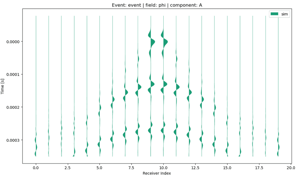
SalvusProject
Fix a bug in plotting shotgathers for single data series.
Example:
p.viz.shotgather(
    data="simulation",
    event="event",
    receiver_field="phi",
    component="A"
)
Salvus version 0.11.43
Released: 2021-10-21
Minor update with a bug fix for serializing cythonized
functions.
SalvusProject
The function serialization can now serialize cythonized functions imported
from other modules.
Salvus version 0.11.42
Released: 2021-10-19
Minor update with some internal changes and
support for frequency domain output in Salvus project.
SalvusProject
Add support for frequency-domain output to Salvus project.
Optional output of the Fourier transform for a discrete set of frequencies
can now be passed as
extra_output_configuration to the launch function.p.simulations.launch( ranks_per_job=4, site_name="local", events=p.events.list(), simulation_configuration="simulation", extra_output_configuration={ "frequency_domain": { "fields": ["displacement"], "frequencies": [1.0, 2.0, 3.0], } }, )
Salvus version 0.11.41
Released: 2021-10-08
This is a large release that adds many features useful for
the inversion of seismic data, particularly for land and near-surface
applications.
SalvusFlow
The observed and synthetic data can now optionally be downsampled before the
misfit and adjoint source are computed. The adjoint source is later upsampled
again and scaled correctly. Useful for expensive misfit functionals.
It can be used either at the event misfit level:
event_misfit = EventMisfit(
    ...,
    # Optionally downsample to the given number of npts.
    max_samples_for_misfit_computation=max_samples_for_misfit_computation
)
Or at the misfit configuration level within SalvusProject:
mc = MisfitConfiguration(
    ...,
    # Optionally downsample to the given number of npts.
    max_samples_for_misfit_computation=max_samples_for_misfit_computation
SalvusMesh
Fix a bug that caused the mesh widget to crash for fields with only negative
values.
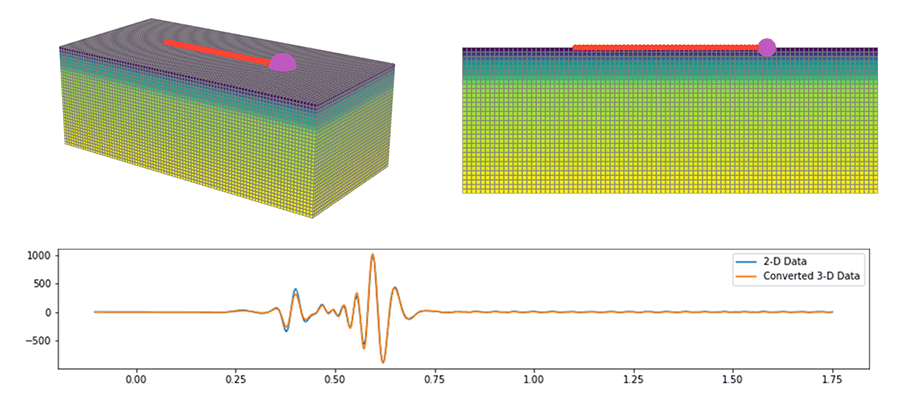
SalvusModules
Added comprehensive support for converting data from a point source to an
equivalent line source which is necessary for example when using 3-D observed
data in 2-D inversions.
We added a variety of different transform, each applicable in different use
cases. Please have a look at the documentation for details.
from salvus.modules.near_surface.processing import convert_point_to_line_source

new_st = convert_point_to_line_source(
    st=st,
    source_coordinates=[22.0, 1.0],
    receiver_coordinates=[132.0, 0.0],
    transform_type="single_velocity_exact",
    velocity_m_s=550.0
)
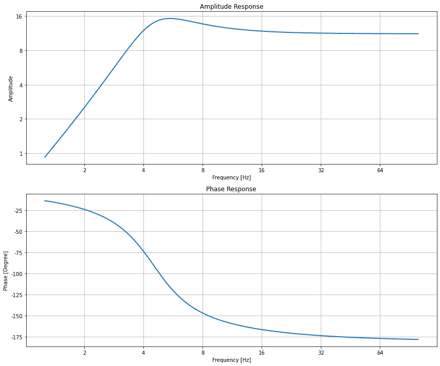
SalvusModules
Added utility functions to compute, remove, and plot geophone responses.
import numpy as np
from salvus.modules.near_surface.processing import geophone_response

frequencies = np.logspace(0.1, 2, 2000)
response = geophone_response.compute_geophone_response(
    frequencies=frequencies,
    geophone_frequency=4.5,
    damping_ratio=0.4,
    calibration_factor=11.2,
)
geophone_response.plot_response(frequencies=frequencies, response=response)
SalvusOpt
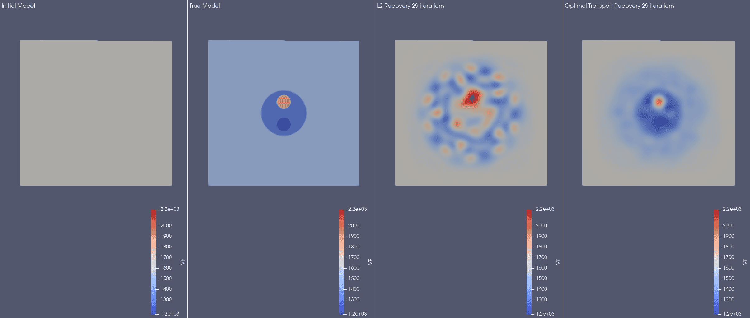
Added an implementation of a graph space optimal transport misfit measure as
introduced in this paper:
L. Métivier, R. Brossier, Q. Mérigot, and E. Oudet. 2019."A graph space optimal transport distance as a generalization of Lp distances: application to a seismic imaging inverse problem"Inverse Problems, Volume 35, Number 8, https://doi.org/10.1088/1361-6420/ab206f
You can use it by choosing
"graph_space_optimal_tranport" everywhere Salvus
accepts misfit functionals. The one tuning parameters is the
"max_expected_time_shift" which, as the name implies, should be set to the
maximum expected time shift in seconds for individual wiggles between observed
and synthetic data.For many problems this can get completely avoid the cycle skipping problem.
This, admittedly manufactured, synthetic inversion example demonstrates the
potential gains:
SalvusProject
The function serialization can now serialize numpy arrays and dictionaries as
closure values.
SalvusProject
Added the ability to use processing fragments to more easily perform some
simple and common processing techniques.
To for example bandpass and normalize some data use
"EXTERNAL_DATA:raw_data | bandpass(1.0, 2.0) | normalize" as the data name.Available processing fragments:
time_shift({SHIFT})normalizescale({FACTOR})flipbandpass({FREQ_MIN}, {FREQ_MAX}[, zerophase][, corners={CORNERS}])
SalvusProject
Added an automatic domain preview visualization for 3-D box domains.

SalvusProject
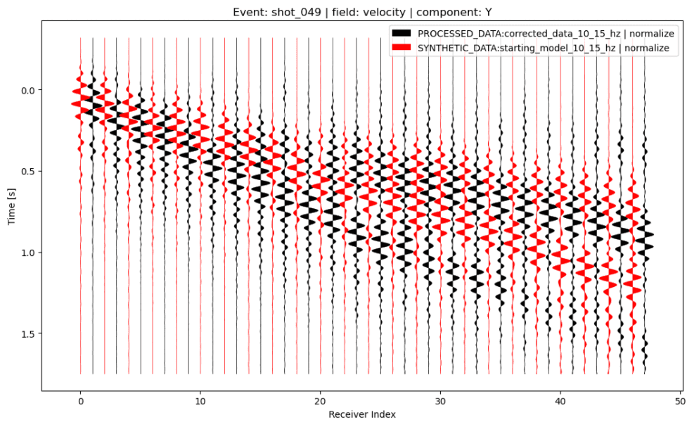
Added an improved shotgather visualization. Amongst other things, it can now
plot interleaved data from multiple traces and sort the receivers with a lambda
function:
p.viz.shotgather(
    data=[
        "PROCESSED_DATA:corrected_data_10_15_hz | normalize",
        "SYNTHETIC_DATA:starting_model_10_15_hz | normalize",
    ],
    event="shot_049",
    receiver_field="velocity",
    component="Y",
    sort_by=lambda r: r.location[0]
)
SalvusProject
Allow for the passing of an interpolation mode to the
mesh_from_xarray
function in the Salvus Toolbox. This allows one to override the default spline
interpolation routine, which may be useful in the presence of strong velocity
contrasts.Salvus version 0.11.40
Released: 2021-09-25
This release contains improvements to the mesh-to-mesh
interpolation implementation, as well as a few fixes and quality-of-life
improvements to SalvusProject functionality and SalvusFlow database handling.
SalvusFlow
All input files are stored in Salvus' internal database. From now on these are
compressed which can safe a lot of space for input files with large number of
receivers. Existing databases will be automatically migrated to the new
structure.
SalvusMesh
Improve the mesh-to-mesh interpolation algorithm by allowing element set to be
further restricted in both the source and destination meshes. This is useful,
for instance, when interpolating between meshes with oceans. Also improved the
heuristic which decided which element to source parameters from if an element
was outside of the mesh or outside of a certain layer set. This should improve
the algorithm's stability in such cases.
SalvusProject
The domain map plots for spherical chunk and UTM domains now automatically zoom
to fit upon loading.
SalvusProject
Less assumptions in the internal layout of AppEEARS DEM files so Salvus now
works with older and newer AppEEARS files.
Salvus version 0.11.39
Released: 2021-09-09
This is a minor release that fixes a bug when applying
anisotropic refinements to the crust in a global domain, and reduces the memory
usage of some SalvusFlow routines.
SalvusFlow
Improve detection of duplicated mesh files when transferring data of JobArrays
to remote sites.
SalvusFlow
Reduce memory usage of
simple_config.Waveform objects by lazy evaluation of
UnstructuredMesh objects.SalvusMesh
Fix a bug where an undefined reference to a refinement skeleton may be deleted
before it was defined.
Salvus version 0.11.38
Released: 2021-08-11
Minor update with some utilities to inspect the contents of a project and
to free up space during an inversion by deleting disposable files.
SalvusProject
Add utility to compress the storage requirements of an
inversion by deleting files which are no longer needed
and/or can be recomputed.
Example:
p.inversions.delete_disposable_files(
  inverse_problem_configuration="my_inversion",
  data_to_remove=["auxiliary", "waveforms", "gradients"]
)
Note that data from the initial model and unfinished iterations
will be kept. It is recommend to remove files in the order
auxiliary, waveforms, gradients, because gradients are the most
expensive to recompute.SalvusProject
Add utility to delete simulation results (waveforms / gradients).
Example:
# Delete waveforms
p.simulations.delete_results(
  simulation_configuration="my_sim_config",
  events=["event"]
)

# Delete gradients
p.simulations.delete_results(
  simulation_configuration="my_sim_config",
  misfit_configuration="my_misfit_config",
  events=p.events.list()
)
SalvusProject
Add utility to list a project's contents.
This function will be called automatically when a project is loaded.
Salvus version 0.11.37
Released: 2021-07-15
This is a small maintenance /bugfix release that primarily serves to activate
2-D fully anisotropic elastic simulations on CUDA-capable GPUs.
SalvusCompute
Activate 2-D fully anisotropic simulations on CUDA capable GPUs, and fixes some
bugs in the associated gradient computations. No API changes are required from
users -- simply feel free to now run 2-D anisotropic simulations and inversions
on a GPU-enabled site!
Salvus version 0.11.36
Released: 2021-07-02
This release adds more flexibility for handling side-set extrusion and
topography in 2-D, as well as a more robust implementation of processing
function serialization. Additionally, the minimum supported CUDA Compute
Capability has been lowered to 3.5, and as such Kepler-based NVIDIA GPUs can
now be used.
SalvusCompute
Previously, the lowest CUDA compute capability supported by Salvus was 6.0, due
to the unavailability of a double precision atomic add function in previous CCs.
A workaround is now implemented, which should allow Salvus to run on GPUs of CC
3.5 and greater. Note that NVIDIA will soon deprecate architectures < 6.0, so at
some point in the future new Salvus versions will again only support CC 6.0 and
greater.
SalvusFlow
Add initial support for the GridEngine job queueing system.
There are a number of different versions of GridEngine out there and minor
adjustments might be necessary for Salvus to run on them. Please let us know if
you encounter some.
SalvusMesh
Add a utility to extrude meshes across side sets in 2D.
The functionality is currently limited to Cartesian meshes and
side sets aligned with a coordinate axis.
Example:
mesh = basic_mesh.CartesianHomogeneousAcoustic2D(
    vp=1500.0, rho=1000.0, x_max=1.0, y_max=0.5,
    max_frequency=1e3,
).create_mesh()

mesh = mesh.extrude_side_set_2D(
    side_set="x1",
    offsets=np.array([0.0, 2.0, 4.0]),
    direction="x",
)
SalvusMesh
More general definition of 2D dem objects for non-spherical models.
Now, y0 can be set to
-np.infty to deform all elements in y direction
with negative y coordinates.Example:
mesh = basic_mesh.CartesianHomogeneousAcoustic2D(
      vp=1500.0, rho=1000.0, x_max=1.0, y_max=2.0, max_frequency=10e3
  ).create_mesh()
  mesh.points[:, 1] -= 0.5
  mesh.add_dem_2D(
      x=np.array([0.0, 1.0]),
      dem=np.array([-0.25, 0.25]),
      y0=-np.infty,
      y1=np.infty,
      kx=1,
      ky=1,
  )
  mesh.apply_dem()
SalvusProject
SalvusProject sometimes has to serialize Python functions to disc (e.g. misfits,
processing functions, ...).
This now works with more functions, like functions that call other custom
functions, closure values within with statements and a few other things.
In general it should just be more reliable.
Salvus version 0.11.35
Released: 2021-06-23
Minor update including small bug fixes and adding support for constant
material parameters per element.
SalvusProject
Small bug fix to visualize 2D box domains without receivers.
Salvus version 0.11.34
Released: 2021-05-28
This release comes with several small fixes and improvements listed below.
New features include built-in support for two new source time functions,
box constraints for inverse problems.
SalvusCompute
Added new gradient output formats
hdf5-full and hdf5-minimal.
hdf5-full contains additional fields stored in the input mesh, e.g., the
index of layers / regions. hdf5-minimal will only write the data fields of
the gradient, but neither coordinates, connectivity nor an xdmf file.The default format
hdf5 remains unchanged.SalvusFlow
Adds two useful built-in source-time functions: a Tone Burst, commonly used to
model ultrasound transducers, and a wavelet with a flattened spectrum, sometimes
used in geophysical applications.
SalvusFlow
Adds a
.to_list() function to all receiver collections so that multiple
collections can more easily be appended to each other.SalvusFlow
Mitigate an error that sometimes happened upon closing the paramiko SSH and SFTP
clients.
SalvusFlow
MPICH sometimes causes a problem on OSX. If this happens during site
initialization the error message now points to the section on the Mondaic
website that describes how to solve it.
SalvusFlow
The source and receiver placement could previously fail for strongly distorted
high-order elements. For these rare cases it now falls back to a slower, more
brute-force method that should always work.
SalvusFlow
Improved the temporal resampling of custom STF functions which is useful for
plotting on the Python side.
SalvusMesh
A list of side sets can now be passed to the
free_surface argument of
AbsorbingBoundaryParameters. These side sets will in turn not be extended with
absorbing layers (if they are requested), and no absorbing conditions will be
placed on them. This is useful, for instance, to model a thing plate
(free_surface=["z0", "z1"]).SalvusMesh
The Jupyter notebook mesh visualization widget now has a "Toggle Mesh" button to
quickly toggle the visibility of the mesh. This is to look at sources and
receivers inside the mesh.
SalvusOpt
Add optional box constraints to the InverseProblemConfiguration and implement
the related projection algorithm for the trust region method.
Here is a snippet that adds lower and upper bounds on VP to an inversion:
mesh = p.simulations.get_mesh("initial_model")
lb = mesh.copy()
lb.elemental_fields["VP"] *= 0.8
lb.elemental_fields["RHO"] *= 0.8

ub = mesh.copy()
ub.elemental_fields["VP"] *= 1.2
ub.elemental_fields["RHO"] *= 1.2

p.inversions.set_constraints(
    inverse_problem_configuration="my_third_inversion",
    constraints={
        "lower_bounds": lb,
        "upper_bounds": ub,
    },
)
SalvusProject
In some rare cases the order of the coordinates in xarray data sets was not
passed on correctly to Salvus' internal interpolation routines. This now works
as expected.
SalvusProject
Deleting a volume, topography, or bathymetry model will now delete any
dependent, auto-generated meshes.
SalvusProject
Make SalvusProject compatible with the latest pyproj 3.1.0 package.
Salvus version 0.11.33
Released: 2021-05-11
This release makes sure Salvus keeps working with the latest versions of
xarray and SQLAlchemy. A consequence of this is that the Python netCDF4
package is now a hard dependency.Please make sure your conda environment/Python installation is up-to-date
before upgrading to this Salvus version.
Additionally this release adds the option to invert for homogeneous material
parameters in the full waveform inversion workflow.
SalvusFlow
Updates to make it work with the latest versions of
xarray and SQLAlchemy.
The netCDF4 package is now a hard dependency which should improve
compatibility when reading and writing files with xarray.SalvusFlow
The
salvus-flow add-site wizard will now also ask if it should
run Salvus using GPUs on a newly configured site.SalvusFlow
Fix a bug in the
SiteNameValidator that caused add-site
to crash when no other site has been initialized yet.SalvusOpt
Extend the mapping function to support inversion for homogeneous models.
Salvus version 0.11.32
Released: 2021-05-05
This release fixes a few minor bugs relevant for regular-grid model extraction,
mesh-to-mesh interpolation, and database management.
SalvusFlow
Salvus now raises an actionable error message in case the internal SQLite
database got corrupted or does not work for another reason.
SalvusMesh
Fix a type issue within
salvus_mesh_utils._match_layers that could
crop up if a mesh was generated outside of SalvusProject.SalvusMesh
Fixes a bug where, in certain exceptional cases,
get_enclosing_elements would
not return the proper reference coordinates.Salvus version 0.11.31
Released: 2021-04-23
This release comes with a new experimental feature for general mesh-to-mesh
interpolations, which is very useful to interpolate the same model between
to different discretizations.
Additionally, we added a workaround for a bug in parallel HDF5 that
sometime occured when reading or writing large datasets.
SalvusCompute
There still seems to be an issue with parallel HDF5 and writing large amounts
of data per rank in HDF5 1.12.0. This patch implements a workaround for
execution on a single rank.
SalvusMesh
Generic mesh-to-mesh interpolation is now implemented in 2- and 3-D! This is
useful in several situations, such as
- representing two models on the exact same mesh,
- increasing the frequency band in an ongoing inversion, and
- re-meshing a model due to a decrease in minimum velocity,
among others. The primary interpolation function is available in
salvus.mesh.tools.transforms. Along with full-mesh interpolations,
layer-to-layer discontinuity-preserving interpolations, and "flattened"
interpolations handling topographic deformations, are supported. Additional
helper functions for re-meshing applications have also been added to
salvus.mesh.salvus_mesh_utils. One of theses is a function to extract
a conservative 1-D model from an unstructured mesh, which helps to ensure that
a new mesh can be generated that respects both the 3-D minimum velocities and
existing discontinuities. Another is a function to match up layers between
two unstructured meshes in the case that their IDs are different. This is
helpful in the case where the interpolation should respect pre-defined
discontinuities in the model.The method currently does not raise if the spatial domains covered by the
target mesh is contained in the source mesh. Use this with care.
For additional information, please see our new tutorial on mesh-to-mesh
interpolations.
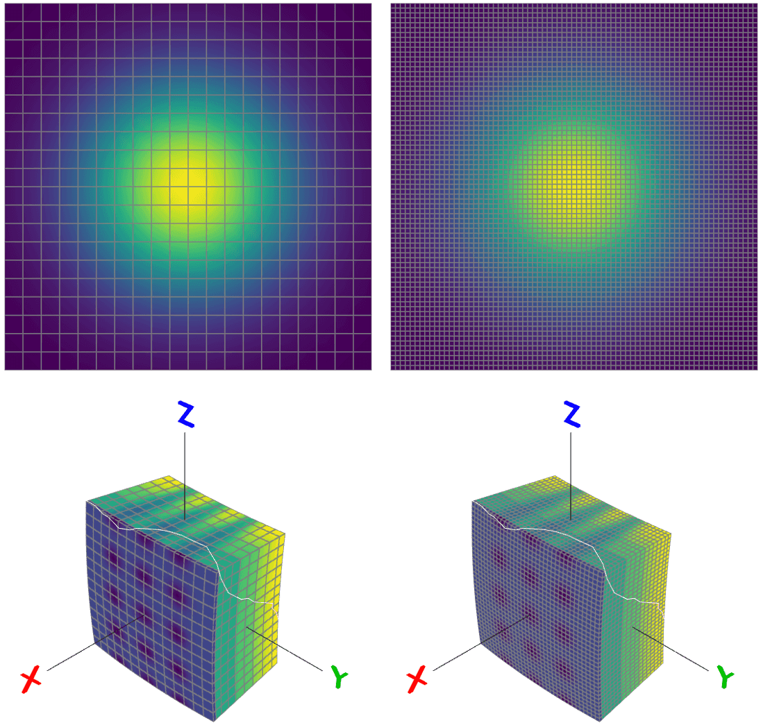
Salvus version 0.11.30
Released: 2021-04-14
This release comes with two main features: (1) better support for spherical
chunk domains formed by arbitrary polygons and (2) a new output format to
compute the wavefield in frequency domain for a set of specified frequencies
by applying the Fourier transform on the fly during the simulation.
Additionally, there are several important bug fixes related to SmoothieSEM
meshes, reading large hdf5 datasets, and writing xdmf files in SalvusCompute.
SalvusCompute
Enable on-the-fly Fourier transforms to output the volumetruc wavefield in
frequency domain for a list of discrete frequencies.
It can be configured in the
simple_config.simulation.Waveform object using
output.frequency_domain.This feature is currently only enabled for simulations on CPUs.
SalvusCompute
Fix a bug in SalvusCompute that caused multiple ranks to write xdmf files.
SalvusCompute
It seems as though the large dataset mitigations introduced in HDF5 1.10.2 were
only applied to dataset writes, and not reads. This introduces a temporary
workaround to read models with large (> 2GB) amounts of data per rank.
SalvusMesh
Fixes an issue that caused broken meshes when smoothiesem was used with high
number of elements in lateral direction.
SalvusProject
Various bug fixes and quality-of-life improvements when using a
SphericalChunkDomain together with a spherical polygon to further constrain
the spatial extent. Most importantly conversions between WGS84 and fully
spherical coordinates are now consistent with the rest of Salvus. The
in-notebook domain plot now also works and shows the original spherical chunk
together with the domain polygon.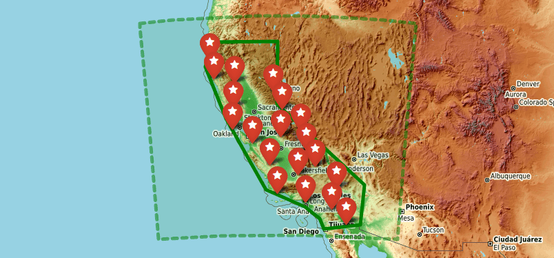
Salvus version 0.11.29
Released: 2021-04-06
Minor release which fixes a bug in certain GPU runs, and adds the capability to
limit the number of simultaneously running jobs in a slurm job array.
SalvusCompute
Fix a bug that previously existed where, in the case of a multi-node GPU run
with 1 rank per node, the GPU halo would not get initialized properly. This
would then lead to a failure during site initialization (as expected).
SalvusFlow
Optionally limit the number of parallel jobs in a slurm job array.
This can be specified in the site configuration of a slurm site with
max_simultaneous_jobs_in_job_array = 4
which internally translates to, for example, the
%4 in --array=0-15%4.Salvus version 0.11.28
Released: 2021-03-19
Minor release including a few bug fixes listed below. Additionally, the
spectral-element order and output sampling rate for receivers is now
configurable through the
WaveformSimulationConfiguration.SalvusFlow
The last part of running a simulation usually is to delete the remote run and
temp directories Salvus needs to simulate waves. In most cases this just
works but especially on network file systems the file system might be busy
and refuse to actually delete anything. Previously this resulted in an
exception but because everything else worked fine this was undesired. It now,
by default, only raises a warning.
You can restore the old behaviour by setting
raise_on_deletion_failure=True
when using the low-level SalvusFlow API calls:sn.api.run(..., raise_on_deletion_failure=True) sn.api.run_many(..., raise_on_deletion_failure=True)
As before it will retry deleting a remote directory up to 5 times before
actually raising the warning or exception with a now slightly increased
timeout between retries.
It will also no longer raise in these cases in SalvusProject which should
make it more stable on some file systems.
Changes to Experimental Features in 0.11.28
SalvusProject
Add the sampling interval for point output to the
WaveformSimulationConfiguration.
SalvusProject
Fix a bug where side-sets involving fluid layers on UTM domains where
incorrectly attached.
SalvusProject
The polynomial degree of the spectral-element basis is now configurable
in the
WaveformSimulationConfiguration.w = WaveformSimulationConfiguration(spectral_element_order=6)
If not specified, the default remains at
4 as in all previous releases.Salvus version 0.11.27
Released: 2021-03-01
The main feature in this release is a new method for the visualization /
analysis of 2- or 3-D models and gradients. The addition of the function
extract_model_to_regular_grid to the salvus.mesh.salvus_mesh_utils
module allows users to regularly sample a given mesh given locations
specified by an xarray dataset. Additional improvements include a more
flexible API for surface topography in UTM domains, a memory use mitigation
when running many shots with the same mesh, and the automatic up-casting of
related types in certain schema (for example: "2 elements per wavelength" is
now upcast to "2.0 elements per wavelength").SalvusFlow
Automatically cast integers to floats in many cases where objects expect
floating point values to be set.
SalvusFlow
Copying simulation objects now, by default, only references a potentially
attached mesh.
Many workflow have a large number of copied simulation objects which can
result in a high memory usage if the meshes are copied as well.
The meshes can still be optionally copied with:
w_copy = w.copy(copy_mesh=True)
SalvusMesh
A new function named
extract_model_to_regular_grid has been added to the
salvus_mesh_utils module. This function performs an interpolation from a
general, unstructured mesh (spherical or cartesian) to a set of points defined
on a xarray dataset. This can be useful, for instance, to create slices
through a model for efficient visualization and analysis. See the function's
docstring for additional examples, information, and tips.Changes to Experimental Features in 0.11.27
SalvusProject
A new parameter can optionally be passed to a cartesian
SurfaceTopography
object that restricts the mesh deformation above a given z-value. This is
useful, for instance, when placing a layer (i.e. the atmosphere) above a free
surface with topography. Related constructors (such as
SurfaceTopography.from_gmrt_file() optionally take this parameter as well.Salvus version 0.11.26
Released: 2021-02-23
This release focusses on quality of life improvements for solving the inverse
problem. It includes a bunch of bug fixes as well as new features.
A new tab has been added to the inversion dashboard showing some
details about model updates and the evolution of the trust-region algorithm.
This grants insights into how an ongoing inversion is doing.
SalvusProject and SalvusFlow can now recover more gracefully from partially
failed job arrays where only a few jobs did not finish.
Furthermore the window picking for seismological full waveform inversions is
now a lot faster.
Note that plotly >= 4.12.0 is required to display the new widgets properly.
To update the python environment, check the installation instructions or run
wget https://mondaic.com/environment.yml -O salvus-0.11.26.yml
conda env update -n salvus -f salvus-0.11.26.yml
.
SalvusFlow
If a few jobs in a Salvus job array failed for some reason, the output for
the successfully completed jobs can now be retrieved in a much simpler way:
SalvusJobArray.copy_output(..., copy_partial_results=True)
copy_partial_results defaults to True.The same parameter is exposed to the
salvus.flow.functions.run_many() command
and also defaults to True there.Changes to Experimental Features in 0.11.26
SalvusOpt
Expose more parameters to steer the adaptive adjustment of the
trust-region radius.
SalvusProject
Bug fix for the gradient widget of the inversion dashboard, where previously
some event-dependent gradients were not displayed correctly.
SalvusProject
Bug fix in the SimulationConfiguration to ensure the
extra_output_configuration passed to launch overwrites additional output
values defined in the WaveformSimulationConfiguration. The output options
in the WaveformSimulationConfiguration will be deprecated in a future
release.SalvusProject
Add a new tab to the inversion dashboard to visualize the progress of
model updates and trust-region radius.
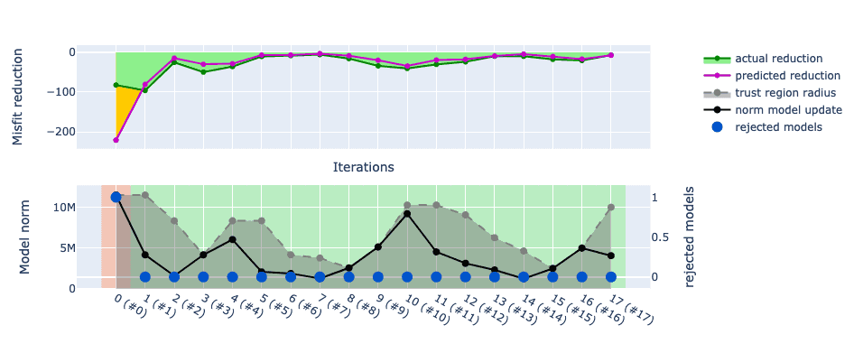
SalvusProject
Add a toggle button to the misfit widget to switch between absolute and
relative misfits - normalized per iteration or event, respectively.
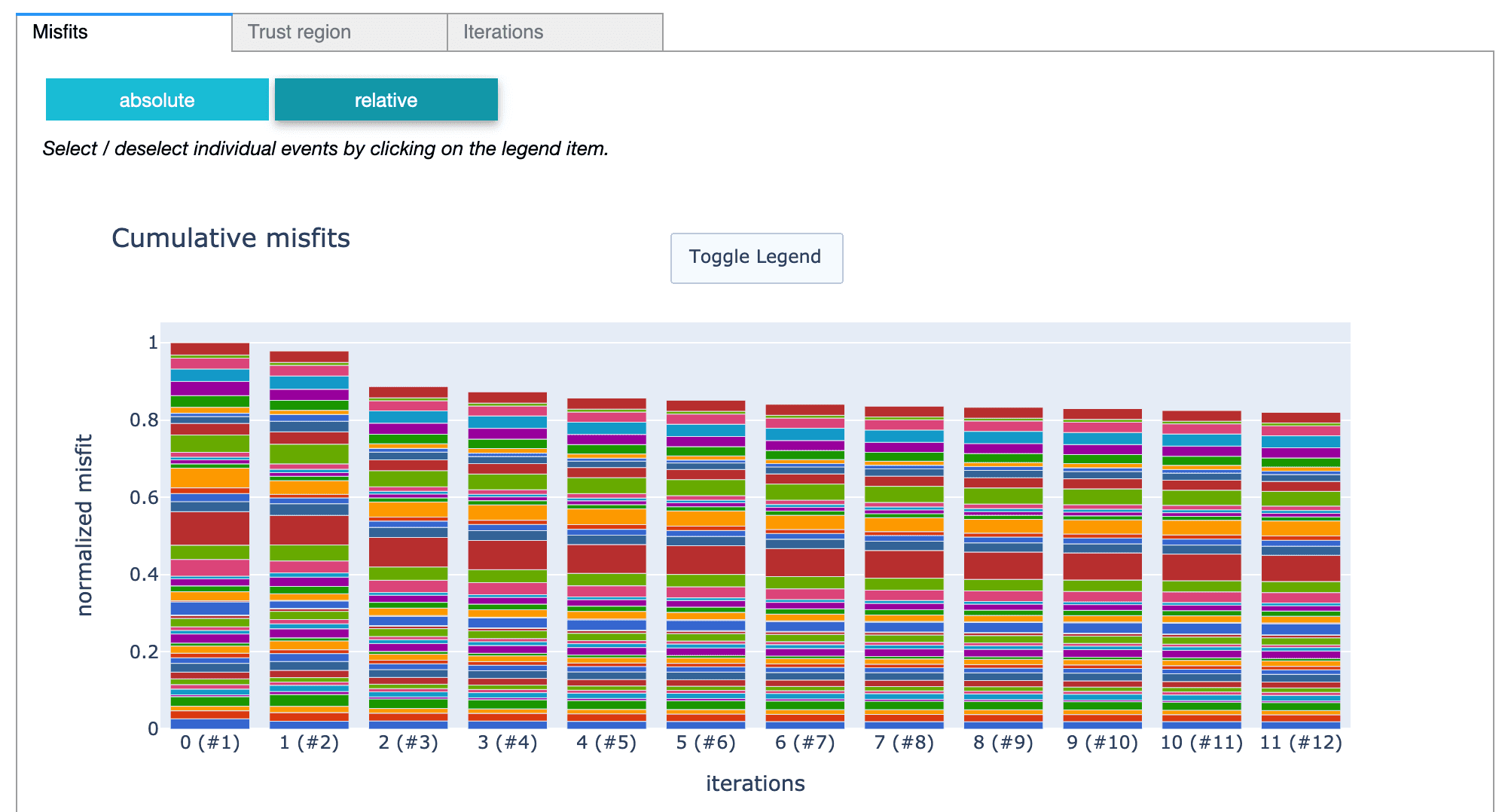
SalvusProject
Much faster seismological window picking for some cases. Additionally it is
now a bit more conservative and will not pick some sketchy windows it did not
pick before. All in all the picked windows should be very similar to results
from the previous version of this algorithm but a few less windows will be
picked.
SalvusProject
The
p.waveforms.has_data() method now also works for synthetic data.SalvusProject
The partial copy of the Salvus job array results has been integrated into all
parts of SalvusProject. If one or more jobs fail for a forward or an adjoint
simulation, it will still raise an exception but copy all successfully
completed jobs to the project folder. Any subsequent simulations launched
will be aware of this and not submit the already run ones.
This makes it much easier to recover from sporadic cluster failures without
having to directly modify the project directory.
Salvus version 0.11.25
Released: 2021-02-12
This release comes with several improvements to make inversions run
more efficiently. New options to manage checkpoints and to reduce the
I/O overhead of smoothing have been added. Furthermore, the mapping function
now offers more general parameterizations.
Additionally, some visualization tools have been improved,
and a tuning parameter to mesh ocean layers was added.
Finally, Salvus now by default supports GLL orders of 1-7.
Additional orders remain available upon request.
SalvusCompute
SEM orders 1-7 are now supported by default for simulation.
Adjoint simulations on GPUs are currently limited to order 4.
SalvusFlow
It is sometimes convenient to visualize source and receiver locations in
Paraview. A new function,
salvus.flow.utils.simulation_src_rec_to_vtk, has
been added to facilitate this. As arguments it takes a simulation.Waveform
object, along with a string specifying what type of entity one wants to
generate a .vtk file for (i.e. source or receiver). Check the function's
docstring for advice on how to open the resultant file in Paraview.SalvusMesh
Adding a new parameter to better control the lateral element size in the ocean.
This is particularly relevant for local domains with strong bathymetry, where
Snel's law in 1D may break down.
SalvusOpt
Reduce the file access of the smoothing algorithms to construct
the diffusion models and enable remote diffusion meshes.
Changes to Experimental Features in 0.11.25
SalvusOpt
Add support for flexible parameter mappings and inversion for
relative or absolute perturbations:
sn.Mapping(
      scaling="relative_deviation_from_prior",
      inversion_parameters=["VSV", "VSH", "VP", "RHO"],
      map_to_physical_parameters={
          "VPV": "VP",
          "VPH": "VP",
      }
  )
The example above assumes a prior model parameterized as
TTI medium. It inverts for four independent parameters that
encode relative perturbations from the prior model.
The deviations in
VPV and VPH are tied to the same
inversion variable VP..SalvusProject
Add
memory_per_rank_in_MB as optional parameter to SiteConfig.
This allows to adjust the memory settings for different machines
during an inversion.SalvusProject
Improve memory management of checkpoints in SalvusProject.
This gives more flexibility to tune the strategy regarding checkpoints.
By default, checkpoints will be stored for every forward run, and
automatically removed after (a) gradients for the simulation configuration
have been computed and/or (b) the model got rejected by the trust region
algorithm.
This behavior can be modified using optional boolean flags
store_checkpoints
and cleanup_checkpoints in the job_submission settings.job_submission={ "forward": ..., "preconditioner": ..., "store_checkpoints": False, "cleanup_checkpoints": False, }
If the former is
False checkpoints will only be stored when gradients are requested. If the latter
is False checkpoints will never be deleted automatically.SalvusProject
The
_plot method of an EventData object now takes an additional optional
parameter: _exclude_cbar. If set to true, a colorbar won't be added to the
axis if a shotgather plot is requested. This makes it easier to produce
shotgathers for multi-component data (i.e. for strain output).Salvus version 0.11.24
Released: 2021-01-12
This release comes with a couple of generalizations and bug fixes related
to preconditioners of the inverse problem as well as utilities to deal with
cylindrical meshes.
Changes to Experimental Features in 0.11.24
SalvusCompute
Fix a bug in the auto time-step detection of the diffusion and the
anisotropic acoustic wave equation that could previously result in a
significant under-estimation of a stable time-step size.
SalvusFlow
New receiver collections to facilitate the creation of 3D apertures
on Cartesian domains.
SalvusMesh
Add utilities to create cylindrical meshes including side sets and
topography.
SalvusOpt
Enable space-dependent smoothing with arbitrary (an)-isotropic
smoothing lengths as preconditioner of an InverseProblemConfiguration.
SalvusProject
Fix a bug in plotting gradients in the inversion dashboard or using
p.viz.nb.gradients.Salvus version 0.11.23
Released: 2020-12-03
This release adds several quality-of-life improvements for ongoing
inversions, as well as a more sophisticated scheme to handle sites where two
factor authentication is required. Support for volumetric models in 2-D
seismological domains was added, along with a relevant tutorial ("Teleseismic
2D"). Volumetric seismological mantle and crustal models will also now
automatically recognize the presence of oceans, and restrict the
interpolation of material parameters to the elastic regions. If more control
over this process is desired, one can still use the
GenericModel
constructor.SalvusFlow
The port number of remote sites in the
~/.ssh/config file is now respected.SalvusFlow
Salvus can now perform interactive SSH logins. This is necessary for example
for interactive two factor authentication schemes.
Enable it like this in the site configuration:
[sites.site_name.ssh_settings]
            hostname = "host"
            username = "user"
            interactive_login = true
Changes to Experimental Features in 0.11.23
SalvusMesh
Adds functionality to refine, increase tensor order or build meshes in chunks
to avoid memory bottlenecks. In particular, this adds two new functions:
Firstly, in
salvus.mesh.tools.transforms uniformly_refine_chunkwise()
wraps uniformly_refine() working with a subset of elements at a time,
writing each of the readily processed chunks to a temporary file and finally
merging everything together. This can both be used to refine each element by
subdivision into an arbitrary number of elements in each dimension and/or to
increase the order of the shape mapping.Secondly,
salvus.mesh.chunked_interface.create_mesh_chunkwise() can be used
instead of create_mesh() of SphericalChunk3D, Cartesian3D and
Cartesian2D using the same approach as described above to directly create
large meshes that would otherwise reach the memory limitations of the
machine.SalvusProject
Enable stopping criteria to limit the maximum number of iterations in an
inverse problem. This is mainly useful for automated monolithic inversion
workflows.
p.inversions.set_stopping_criteria(
  inverse_problem_configuration="...",
  criteria={
    "max_iterations_global": 10,
    "max_iterations": 5,
  }
)
The criteria can be overwritten anytime to continue with the inversion.
global settings apply to the entire inversion tree, the other settings
apply to individual branches.SalvusProject
Remove some path dependencies which previously prevented renaming the project.
SalvusProject
Various improvements to make 2-D seismological domains more useful.
SalvusProject
The interpolation of volumetric models onto seismological meshes was
previously only available for 3-D domains. Support is now extended to 2-D
domains, with "longitude" and "radius" OR "depth" being required coordinate
axes in the parent xarray Dataset. A new tutorial (
teleseismic_2d) has been
added, fleshing out this feature.SalvusProject
Add the ability to ignore elements flagged with a certain value during volume
model interpolation for seismological models. This is useful, for instance,
if one wants to limit interpolation to a specific region (say, the elastic
subsurface, and not any water layers). See the description in the seismology
GenericModel constructor for more details. Crustal and Mantle models will
now ignore fluid elements by default, to ensure that elastic models are not
interpolated into oceans. Is this behavior is undesirable, one has more
control with the GenericModel interface.Salvus version 0.11.22
Released: 2020-11-10
This release contains several small improvements to streamline the workflow
orchestration behind the scenes.
SalvusFlow
API CHANGE
Salvus uses a job database to keep track of asynchronously launched jobs.
Over time this database can become quite big to the point of negatively
effecting the total performance.
With this change Salvus will now perform periodic maintenance of the database
to optimize it and keep its size in check.
Additionally finished jobs are no longer moved into the "archived" group in
the database but removed from the database upon job deletion. We don't expect
this to have an effect on any user.
Changes to Experimental Features in 0.11.22
SalvusOpt
Provide a workaround for externally computed and incorrect adjoint sources.
It is strongly recommend to verify the implementation of custom misfits and
adjoint sources with a finite-difference test.
Using the optional parameter
force_trust_region_scaling badly scaled
adjont sources can be mitigated by enforcing to scale the proposed model
update to the trust region radius.SalvusProject
When re-launching simulations for which data already exist
(e.g. to compute checkpoints), previously computed outputs are kept in the
project file structure and only overwritten once the new jobs have finished.
Additionally, a utility to manually clean the simulation store has been added.
Salvus version 0.11.21
Released: 2020-11-05
This release contains several quality of life improvements and fixes for some
minor issues.
SalvusFlow
The site configuration for local and SSH sites now has an extra
python_binary key to choose which Python is used to execute the minimal
wrapper script used to launch and control SalvusCompute. This is only
important for sites which do not have a Python on their default paths.Usage:
[sites.laptop]
    ...
    [sites.laptop.site_specific]
    python_executable = "/usr/local/bin/python"
SalvusFlow
Salvus now supports usernames in SSH proxy jump connections with settings like
ProxyJump user@hostname in ~/.ssh/config files.SalvusFlow
A full disk previously raised an error that the internal SalvusFlow
database was corrupt. It now gives a more descriptive error message.
SalvusFlow
salvus-flow init-site SITE_NAME now always prints the disk usage of the
Salvus controlled run and temp directories. As init-site is called each
time Salvus is upgraded this serves as a period reminder to monitor the size
of these directories.Changes to Experimental Features in 0.11.21
SalvusProject
The internal workflow for handling checkpoints and adjoint simulations has
been improved to avoid duplicated simulations for missing checkpoints on
remote sites. This changes the hash values of adjoint simulations, which do
not depend on synthetic receiver files anymore.
SalvusProject
The waveform plotting widget can now also plot windows without a reference
time.
Salvus version 0.11.20
Released: 2020-10-25
This release brings in local refinements for cylindrical meshes, a speed-up
for surface data output, and several usability improvements in SalvusProject.
See below for a detailed list of features and bugs that have been patched.
SalvusCompute
Fixed the applications of pressure-free boundaries for GPU simulations in
certain situations where refinements were present along fluid/solid coupling
interfaces.
SalvusCompute
Significant speedup to the detection of which facets to select for surface
output.
SalvusMesh
API CHANGE
Add cylindrical interpolation to local refinement schemes and adopt same
interface as change_tensor_order() has for interpolation_type. This changes the
api for spherical interpolation from
m.refine_locally(mask, spherical=True, r0_spherical=1.0, r1_spherical=2.0)
to
m.refine_locally(
    mask,
	interpolation_mode="spherical",
	interpolation_kwargs={"r0_spherical": 1.0, "r1_spherical": 2.0}
)
The new cylindrical scheme can be used accordingly
m.refine_locally(
    mask,
	interpolation_mode="cylindrical",
	interpolation_kwargs={"r0_cylindrical": 1.0, "r1_cylindrical": 2.0}
)
Below an example of how this can be used for improved representation of
cylindrical structures (left new, right old).
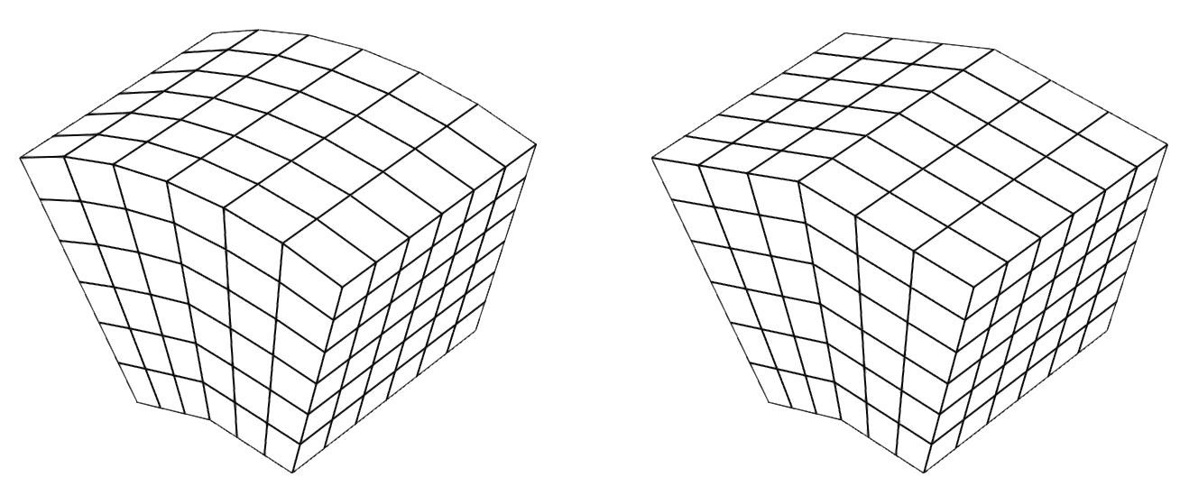
Changes to Experimental Features in 0.11.20
SalvusOpt
Improve the inversion tree widget to visualize per-branch progress.
SalvusProject
The
p.simulations.launch() method can now take extra output configurations.
These can be any setting that does not modify the receiver output which
currently are surface and volume data settings as well as the memory per rank
buffer settings.p.simulations.launch( simulation_configuration="basic", events=p.events.list(), site_name="my_computer", ranks_per_job=12, extra_output_configuration={ "volume_data": { "sampling_interval_in_time_steps": 50, "fields": ["displacement"], }, "surface_data": { "sampling_interval_in_time_steps": 20, "fields": ["acceleration", "velocity"], "side_sets": ["x0", "x1"], }, "memory_per_rank_in_MB": 2000.0, }, )
SalvusProject
The
Project.from_domain() constructor now takes an optional argument
load_if_exists which defaults to False. If this is set to True, and if
the domains are identical, future runs of this constructor will simply load
the existing project from disk rather than raising a "project already exists"
error. This helps remove some boilerplate code which the user previously had
to write.SalvusProject
Add widget to query status of simulations and and improve the widgets of
waveforms and inversions.
SalvusProject
Minor bug fix in visualizing 2D domains using
p.viz.nb.domain that did not
display some source types correctly.Salvus version 0.11.19
Released: 2020-10-05
Minor update that enables license tokens for the diffusion equation.
Furthermore, it adds some utilities to handle remote data in SalvusProject
as well as small bug fixes listed below.
Changes to Experimental Features in 0.11.19
SalvusMesh
Fixing a bug where an anisotropic refinement is used in a single layer spherical model.
SalvusProject
Previous to this change, the parameters governing the behavior of the linear
solids in viscous simulations would only be properly attached if they came in
via a background model. Now these parameters can be supplied to a
ModelConfiguration via the LinearSolids class (which can be found in
salvus.namespace). Additional validations and checks have also been added
to help the user when viscous simulations are either requested or thought to
be desired.SalvusProject
Automatically clean-up checkpoint files after an adjoint simulation.
SalvusProject
Add utilities to handle remote output data and to manually delete jobs
in SalvusProject.
SalvusProject
Chaining processing function in SalvusProject now works as expected.
Salvus version 0.11.18
Released: 2020-09-29
Minor update with a couple of bug fixes listed below as well as
improved compatibility with
xarray > 0.16.0.SalvusFlow
Fixed a bug where in some specific cases it might have requested windows and
weights for components that do not have synthetic data and thus failed.
Changes to Experimental Features in 0.11.18
SalvusOpt
Fix the description in the caption of time-frequency phase shift plots.
SalvusProject
Fix a bug in the horizontal spacing when generating 2D layered meshes from
splines and extruding horizontally for absorbing boundaries.
Salvus version 0.11.17
Released: 2020-09-18
This release contains improvements in a number of different areas.
Salvus can now compute consistent adjoint sources for measurements on the
time derivative fields, e.g. adjoint sources for receivers recording
velocity and phi_t. Additionally the (time frequency) phase misfits have
seen some significant improvements and added flexibility.On the model building side there is a new function to derive a 1-D background
model required for meshing from 2- or 3-D Cartesian volumen models.
Aside from that there are a few minor additions and bugfixes, please refer to
the full changelog for details.
SalvusFlow
Add a new Cartesian receiver collection which creates a 2-D array of side set
receivers for use with 3-D models. The presence of a
"z1" side-set is
assumed, and the receivers will be buried exactly depth_in_meters meters
below this side-set.SalvusFlow
A minimal taper (the first and last 5 samples) will now be applied to every
waveform trace before the misfits and adjoint sources are computed in the
EventMisfit object. This should not have any (or only a very minimal) effect
on existing inversions but is more stable in certain edge cases.SalvusFlow
The
EventMisfit object can now compute fully consistent adjoint sources for
measurements on receivers recording velocity or phi_t with any misfit
functional. This functionality is also available from within SalvusProject.SalvusMesh
Fix a bug where 1 layer of boundary elements would be added to a Cartesian
mesh, even if an absorbing boundary width of 0 meters was requested.
Changes to Experimental Features in 0.11.17
SalvusOpt
The phase misfit now does a better selection of which frequencies to use. One
can control which frequency to use and the minimum energy level of the
frequencies to use for the phase difference measurement.
from salvus.opt.misfits import get_misfit_function

misfit, adjoint_source = get_misfit_function("phase_misfit")(
    data_observed=data_observed,
    data_synthetic=data_synthetic,
    sampling_rate_in_hertz=sampling_rate_in_hertz,
    frequency_limits=(0.1, 0.5),
    # These two are optional.
    absolute_value_threshold=1e-3,
    taper_type="hanning",
)
The old implementation is still valid (but not recommended) and can be
accessed with
get_misfit_function("phase_misfit", version=1)
Existing projects that used the old phase misfit will keep using it until a
new
MisfitConfiguration has been created.SalvusOpt
Fixed a bug in the adjoint source scaling of time-frequency adjoint sources
that occurred for phase-shifted signals.
Additionally the time frequency phase misfit is now a lot more flexible with
more options.
from salvus.opt.misfits import get_misfit_function

misfit, adjoint_source = get_misfit_function("time_frequency_phase_misfit")(
    data_observed=data_observed,
    data_synthetic=data_synthetic,
    sampling_rate_in_hertz=sampling_rate_in_hertz,
    # These two are mandatory.
    segment_length_in_seconds=15.0,
    frequency_limits=(0.1, 0.5),
    # The others are optional.
    segment_overlap_fraction=0.75,
    absolute_value_threshold=1e-3,
    taper_type="hanning",
    stft_window="hann",
)
SalvusProject
Add a function
derive_bm_file() to derive a 1-D background model from a 2-
or 3-D Cartesian volume model. This is useful, for instance, when the 3-D
model has a significant increase in velocity with depth, and when no
appropriate 1-D model exists a-priori. If the velocity profile allows, using
the 1-D model output by this function may result in the insertion of doubling
layers when a simulation mesh is created, and as a consequence may allow for
a reduction of computational cost.SalvusProject
API CHANGE
Minor modifications to
create_events_from_segy_file to handle 2-D events.Salvus version 0.11.16
Released: 2020-09-08
This release comes with several improvements regarding data selection and
inverse modeling.
There are no breaking changes in the stable API.
However, the window selection in SalvusProject has been completely rewritten,
and is not compatible with previous versions.
The new
DataSelectionConfiguration allows window- and station-dependent
weights. Furthermore, there are several new options for visualization and
quality control of misfits. See the Seismological Gradient tutorial in the
Experimental section for several examples.The mapping function has been extended to offer built-in support for a region
of interest, and event-dependent masking of sources and receivers to mitigate
singularities in the sensitivity kernels.
A new function for uniform mesh refinement and model interpolation has been
added to
SalvusMesh.There are several more small changes documented below.
SalvusFlow
Added a new low level
EventWindowAndWeightSet class. It is a per-event data
structure that can be serialized to disc that is able to store interval
windows (e.g. windows that have a start as well as an end time). Additionally
it can store weights at the receiver, component, as well as the individual
window level.In most cases this will be utilized through SalvusProject but it can be
used outside of it and it directly integrates with SalvusFlow's
Event and
EventMisfit infrastructure.SalvusMesh
Added ability to create SmoothieSEM meshes with surface as well as Moho
topography, ellipticity and ocean loading. Includes several minor bugfixes
to the SmoothieSEM meshes introduced in the previous release.
sm = sn.simple_mesh.SmoothieSEM()

sm.basic.model = "prem_iso_one_crust"
sm.basic.min_period_in_seconds = 200.0
sm.basic.elements_per_wavelength = 2.0
sm.basic.number_of_lateral_elements = 2

sm.advanced.tensor_order = 4

sm.source.latitude = 38.82
sm.source.longitude = 40.14

# Ellipticity.
sm.spherical.ellipticity = 0.0033528106647474805

# Surface topography.
sm.topography.topography_file = "topography_earth2014_egm2008_lmax_256.nc"
sm.topography.topography_varname = (
    "topography_earth2014_egm2008_lmax_256_lmax_16"
)

# Moho topography.
sm.topography.moho_topography_file = "moho_topography_crust_1_0_egm2008.nc"
sm.topography.moho_topography_varname = (
    "moho_topography_crust_1_0_egm2008_lmax_16"
)

# Ocean loading.
sm.ocean.bathymetry_file = "bathymetry_earth2014_lmax_256.nc"
sm.ocean.bathymetry_varname = "bathymetry_earth2014_lmax_256_lmax_16"
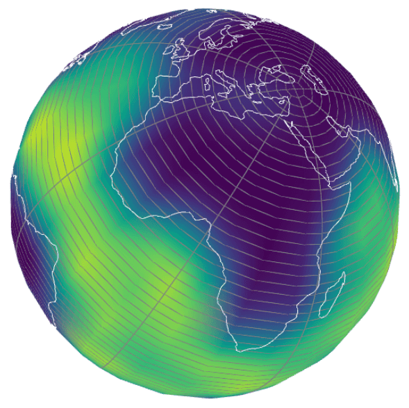
SalvusMesh
Added a function to uniformly refine any mesh to double its element count
along each dimension and thus doubles its resolved frequency. This should
work for arbitrarily complicated meshes including discontinuities. Material
parameters will be interpolated onto the new elements.
from salvus.mesh.tools.transforms import uniformly_refine

new_mesh = uniformly_refine(mesh, tensor_order=2)
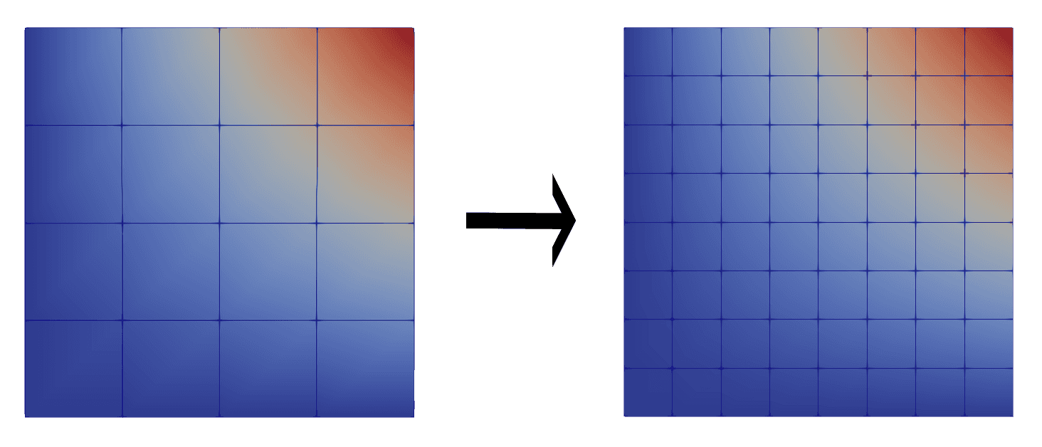
Changes to Experimental Features in 0.11.16
SalvusCompute
Include the reference frame in the HDF5 gradient output files.
SalvusOpt
Added features for defining a region of interest and for
cutting around sources and receivers in the adjoint mapping
function.
SalvusProject
Implement
p.viz.nb.domain() method for 2D box domains.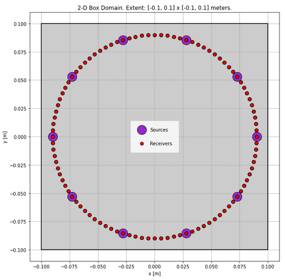
SalvusProject
Move job submission settings to the InverseProblemConfiguration and
enable different site configurations for simulations and the preconditioner.
The previous way of providing
site_name, ranks_per_job and
wall_time_per_job_in_seconds through the iterate and resume functions
still work, but will be deprecated in the future.SalvusProject
Add interactive misfit plots to the inverse problem Jupyter notebook widget.
SalvusProject
Better workflow management for misfit and gradient computations.
The newly added functionality ensures consistent settings for site name
and the number of ranks and automatically resubmits simulations if the
checkpoints are no longer available.
SalvusProject
With very large models and / or meshes, interpolating volumetric models can
take some time. Here a 'verbose' argument is now accepted by
toolbox.interpolate_spherical, which will print a progress bar if the
verbosity is 1 or greater. The verbose behavior is the default when
generating spherical meshes with project.SalvusProject
Better error handling and management of entities using
UnstructuredMeshSimulationConfiguration objects.SalvusProject
Adding an already existing inverse problem configuration again with exactly
the same parameters will no longer throw.
SalvusProject
API CHANGE
Projects created with an older Salvus version using the
windows component
cannot be imported anymore.The
windows component has been removed in favor of a more generic
DataSelectionConfiguration. This is for one more in line with the rest of
SalvusProject but also more powerful and flexible.A direct consequence is that any function or object that took a
window_set_name argument now takes a data_selection_configuration
argument.A
DataSelectionConfiguration is either a function that is applied on the
fly to select pieces of data (think generalized windows and weights) or one
EventWindowAndWeightSet set per event (or a combination of both).Projects that used an on-the-fly temporal weighting/windowing function now have
to use it by creating a new
DataSelectionConfiguration with an attached
data_selection_function. The function itself does not have to be changed.p.add_to_project( sn.DataSelectionConfiguration( name="mute_with_direct_phase", receiver_field="phi", data_selection_function=mute_with_direct_phase, ) )
The
pick_windows() seismological action also requires changing
window_set_name to data_selection_configuration (if that configuration
does not yet exist, it will be created). In addition the
window_taper_width_in_seconds argument is now exposed and required. It
controls the width of the taper for the windows.p.actions.seismology.pick_windows( data_selection_configuration="custom_windows", ... window_taper_width_in_seconds=10.0, )
Salvus contains a lot of convenience functions to pick windows and weight
individual receivers but it is also possible to directly operate on these
data structures for full control.
# Get the data selection configuration.
dsc = p.entities.get(
    entity_type="data_selection_configuration", entity_name="custom_windows"
)
# If interval windows have been picked before an event, its
# `EventWindowAndWeightSet` can be retrieved.
ewws = dsc.get_event_window_and_weight_set(event=p.events.get("event_0000"))
This can than be used to exert detailed control on everything. Once this has
been done it will be applied in all subsequent steps that utilize that
particular
DataSelectionConfiguration.In [1]: ewws.receivers Out [1]: {'XX.A0000.': {'receiver_weight': 1.5462720296177797, 'components': {'Z': {'component_weight': 1.0, 'windows': [{'window_start': 229.67554, 'window_end': 1389.219377, 'window_weight': 1.0}]}, ... In [2]: ewws.receivers["XX.A0000."]["receiver_weight"] = 0.7 In [3]: ewws.write(overwrite=True)
SalvusProject
Can now add weights to individual receivers and components which will then be
applied to each misfit and adjoint source computation. This could have been
previously done with a custom windowing function with weights but this is
more convenient and easier to control. It is detailed in other changelog
items of this release.
It can either happen via window picking and receiver weighting or directly in
the data selection function:
def data_selection_function(st, receiver, sources):

    # Receiver and component weights.
    weights = {
        # This is optional but allows to specify additional weights
        # important for the misfit and adjoint source computations.
        "receiver_and_component_weights": {
            # Pass the receiver weight here.
            "receiver_weight": 0.75,
            # It is also possible to give weights to individual
            # receivers.
            "component_weights": {"X": 1.0, "Y": 0.8, "Z": 0.5},
        }
    }

    for tr in st:
        component = tr.stats.channel[-1]
        temporal_weights = compute_window(...)

        # Individual window weights.
        weights[component] = [
            {"values": temporal_weights, "misfit_weight": 0.8},
            ...
        ]

    return weights

# Add to the project.
p.add_to_project(
    sn.DataSelectionConfiguration(
        name="custom_data_selection",
        receiver_field="phi",
        data_selection_function=data_selection_function,
    ),
    overwrite=True,
)
SalvusProject
Added implementations for a few common seismological receiver weighting
schemes with a general and easy to extend interface.
# Custom receiver weighting function.
def my_favorite_station(event, receivers, receiver_name):
    weights = {}
    for name in receivers:
        if name == receiver_name:
            weight = 2.0
        else:
            weight = 1.0
        weights[name] = weight
    return weights


p.actions.seismology.add_receiver_weights_to_windows(
    # Add the weights to existing windows in this data selection
    # configuration.
    data_selection_configuration="custom_windows",
    events=p.events.list(),
    # The weights for each item in the chain will be multiplied together.
    weighting_chain=[
        {
            "weighting_scheme": "ruan_et_al_2019",
            "function_kwargs": {"ref_distance_condition_fraction": 1.0 / 3.0},
        },
        {
            "weighting_scheme": "mute_near_source_receivers",
            "function_kwargs": {
                # All receivers closer than this to the sources
                # will have zero weight.
                "minimum_receiver_distance_in_m": 200e3,
                # All receivers further away than this will not be muted.
                "maximum_receiver_mute_distance_in_m": 1000e3,
                # How to go from weight 0 to weight 1 for receivers in the
                # transition region. Currently only "hanning" is supported.
                "taper_type": "hanning",
            },
        },
        # Custom weighting function.
        {
            "weighting_scheme": my_favorite_station,
            "function_kwargs": {"receiver_name": "XX.A0044."},
        },
    ],
    # Normalize the sum of all receiver weights to the receiver count.
    normalize=True,
)
SalvusProject
New seismological receiver weight map plot.
p.viz.seismology.receiver_weights_map(
    data_selection_configuration="custom_windows"
)
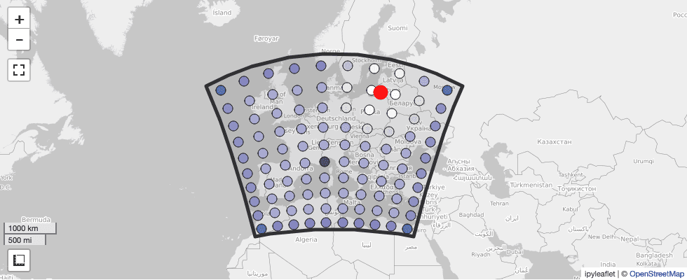
SalvusProject
Various part of SalvusProject can serialize functions to disc. This is now
more powerful and easier to use as the serialized functions can now access
closure values as well as other variables in the global scope of the
functions which will also be serialized alongside. Thus external variables
and imports will now work with these functions.
Basically it means that it should now just work in more cases without any
extra work or rewrites.
SalvusProject
The
p.viz.seismology.misfit_map() method is now a widget and the event can
be selected interactively. Thus passing the event argument is no longer
necessary.SalvusProject
New method to visualize and compare histograms of misfits.
p.viz.misfit_histogram(
    simulation_configuration_a="initial_model_70_120_seconds",
    simulation_configuration_b=p.inversions.get_simulation_name(
            inverse_problem_configuration="inversion", iteration_id=25
    ),
    misfit_configuration="phase_misfit_70_120_seconds",
    events=p.events.list(),
    merge_all_components=False
)
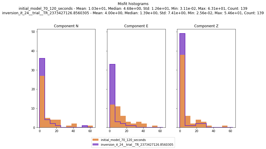
SalvusProject
A few new utilities to analyze the statistics of interval windows.
One is the ability to get a
pandas.DataFrame object containing statistics
about all windows for a list of events. This is very useful to do some custom
analysis and figure out which events to use in the final inversion.df = p.entities.get( entity_type="data_selection_configuration", entity_name="selection_a" ).get_interval_window_statistics_table(events=p.events.get_all())
A styled version of this table with all events in a project can be visualized
with:
p.viz.interval_window_statistics("selection_a")
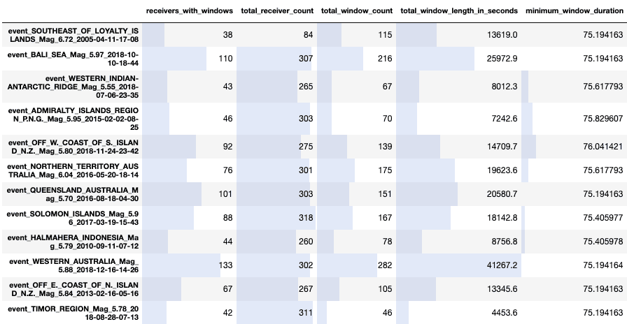
Salvus version 0.11.15
Released: 2020-08-13
This release features a revamp of the mesh masking interface to be more
flexible as well as easier to use. Additionally it contains a first version
of global and continental scale wavefield adapted SmoothieSEM meshes.
Furthermore it includes a new receiver collection and the ability to retrieve
detailed misfit information from an
EventMisfit object. Last but not least
it includes a bugfix for gradients in meshes employing the region-of-interest
feature while using nontrivial checkpoints.For the experimental SalvusProject packages it contains a number of
quality-of-life to visualize and understand misfits in more detail as well as
a number of bugfixes and some polish.
This update has no user facing breaking changes (aside the mesh masking) so
we recommend this update to all users.
SalvusCompute
Bugfix for the region of interest in adjoint runs with nontrivial checkpoints.
SalvusFlow
New
EventMisfit.misfit_per_receiver_and_component_and_weight_set attribute
to yield a more detailed view of how the misfit for a single event is
computed.In [1]: ed.misfit_per_receiver_and_component_and_weight_set Out [1]: {'XX.A0000.': {'Z': [0.00088682823102153761], 'N': [0.000256782248385296], 'E': [0.00012302960702887129, 0.0004303495400]}, 'XX.A0001.': {'Z': [0.0010641578304181843], 'N': [0.00025058292454050639], 'E': [0.00012369945631215902]}, ... }
SalvusFlow
New
simple_config.receiver.seismology.collections.SideSetGridPoint3D
receiver collection.lat_c, lon_c = 45.0, 10.0 lat_e, lon_e = 15.0, 18.0 receivers = sn.simple_config.receiver.seismology.collections.SideSetGridPoint3D( lat_center=lat_c, lat_extent=lat_e * 0.9, lon_center=lon_c, lon_extent=lon_e * 0.9, fields=["displacement"], n_lat=10, n_lon=10, )
SalvusMesh
New method
UnstructuredMesh.get_side_set_nodes() to get all nodes in a side
set.SalvusMesh
API CHANGE
New mask generators (
SurfaceMaskGenerator, RayMaskGenerator) replacing
the existing JSON based masking interface.They are now applied via the
processing_function argument to the
central run_mesher() function.We expect this to only affect a small number of users.
SalvusMesh
Added the ability to generate wavefield adaptive spectral-element meshes
which we refer to as
SmoothieSEM.sm = sn.simple_mesh.SmoothieSEM() sm.basic.model = "prem_iso_one_crust" sm.basic.min_period_in_seconds = 200.0 sm.basic.elements_per_wavelength = 2.0 sm.basic.number_of_lateral_elements = 4 sm.advanced.tensor_order = 2 sm.source.latitude = 35.0 sm.source.longitude = 12.0
Changes to Experimental Features in 0.11.15
SalvusProject
Warn when receiver fields other than
"displacement" or "phi" are used in
a MisfitConfiguration object. Otherwise the adjoint sources are currently
not fully consistent.SalvusProject
New
p.misfits.get_misfit_comparison_table() method yielding a
pandas.DataFrame containing detailed per-receiver misfit information that
can be used for further custom analysis.In [1]: p.misfits.get_misfit_comparison_table( reference_data="initial_model", other_data=[ p.inversions.get_simulation_name( inverse_problem_configuration="inv", iteration_id=4 ) ], misfit_configuration="L2-misfit-to-target-model", event="event_0000", ) Out [1]: initial_model (ref) inv_it_3__trial Reduction inv_it_3__trial XX.A0000. 1.266640e-03 0.000224 0.001043 XX.A0001. 1.438440e-03 0.000361 0.001078 XX.A0002. 1.450685e-03 0.000369 0.001081 XX.A0003. 1.607995e-03 0.000430 0.001178 XX.A0004. 9.473526e-04 0.000238 0.000709 ... ... ... ... XX.A0095. 1.182061e-05 0.000065 -0.000053 XX.A0096. 1.360653e-06 0.000529 -0.000527 XX.A0097. 9.762485e-07 0.000102 -0.000101 XX.A0098. 4.663780e-06 0.000306 -0.000301 XX.A0099. 1.784453e-06 0.000165 -0.000163 [100 rows x 3 columns]
SalvusProject
New
p.viz.nb.misfit_comparison() method to display the output from the
p.misfits.get_misfit_comparison_table() method in a pretty table.p.viz.nb.misfit_comparison( reference_data="initial_model", other_data=[ p.inversions.get_simulation_name( inverse_problem_configuration="inv", iteration_id=4 ) ], misfit_configuration="L2-misfit-to-target-model", event=p.events.list()[0], )
SalvusProject
New
p.viz.seismology.misfit_map() method to display the output from the
p.misfits.get_misfit_comparison_table() method on a geographical map.p.viz.seismology.misfit_map( reference_data="initial_model", compare_data=p.inversions.get_simulation_name( inverse_problem_configuration="inv", iteration_id=5 ), misfit_configuration="L2-misfit-to-target-model", event=p.events.list()[0], )
SalvusProject
Can now delete entities, even if they cannot be instantiated anymore. Useful
for certain edge cases.
SalvusProject
Fully consistent
is_point_in_domain() check for spherical chunk domains.SalvusProject
The map visualization for spherical chunks now also works for domains
crossing the international date line.
sn.domain.dim3.SphericalChunkDomain(
    lat_center=52.0,
    lat_extent=16.0,
    lon_center=170.0,
    lon_extent=66.0,
    radius_in_meter=6371000.0,
).plot()
Salvus version 0.11.14
Released: 2020-07-29
This release contains a few minor user facing improvements for the stable
part of Salvus but it largely focusses on improvements for the experimental
SalvusProject module.
The release is fully backwards compatible so we recommend all users to
update.
SalvusCompute
All wavefield outputs now have a
reference_time_in_seconds attribute. Thus
also receiver output in the HDF5 block format can now be absolutely located
in time and not just ASDF files.SalvusFlow
The
EventData object will now raise an exception if a temporal weight
function returns components that the data cannot have.SalvusMesh
Fix the ABC element field for zero-width absorbing boundaries for proper
visuzliations. This only affected visualizations and had no effect on the
simulations.
SalvusMesh
Slider to change the min/max values of the colormap in the Jupyter notebook
mesh visualization widget.
Changes to Experimental Features in 0.11.14
SalvusOpt
Generic mapping interface to transform inversion models between physical and
simulation space.
SalvusProject
A few quality-of-life improvements for inversions.
SalvusProject
Uppercase variables names during model interpolation from xarray data sets
and NetCDF files. Thus lowercase case variables now also work.
SalvusProject
Several improvements and small bug fixes in a number of Jupyter notebook
inversion widgets.
SalvusProject
New inversion action to faciliate model smoothing.
p.actions.inversion.smooth_model(
    model=gradient,
    smoothing_configuration=sn.ConstantSmoothing(
        smoothing_lengths_in_meters={"VP": 0.01, "RHO": 0.01,},
    ),
    ranks_per_job=4,
    site_name="local",
)
SalvusProject
Enable misfit configurations without observed data.
SalvusProject
Prevent processing/misfit functions that cannot be deserialized again from
being stored in a project in the first place.
SalvusProject
New experimental 2-D circular domain.
Changelog for Older Versions
Released: July 16th 2020
Changes:
SalvusMesh: Fix side-sets for masked global domains.SalvusCompute: Minor bug fix for safely writing the meta json.SalvusCompute: Auto-time-step detection for the diffusion equation.SalvusFlow: Removed thecpu_countargument from all functions performing receiver/source placement. It was not actually any faster and we have to re-evaluate the chosen approach.SalvusFlow: More control over the end time when using aFilteredHeavisidesource time function.SalvusFlow: TheFilteredHeavisideSTFs now defaults to 3 lowpass filter corners and additionally allows explicitly settings the sampling rate. changed defaults
Experimental features:
SalvusOpt: New implementation of time-frequency phase misfits.SalvusOpt: Added new phase misfit.SalvusOpt: Bug fix for scaling of cross-correlation adjoint sources.SalvusProject: Correctly plot the time axis for seismological data.SalvusProject: More stable and informative window picking process.SalvusProject: Statistical window visualizations.SalvusProject: The window picking action can now work with external window picking functions. API changeSalvusProject: Function serialization now works with imports as well as closure variables making it a lot more flexible.SalvusProject: The window picking action can now optionally also only act on a subset of receivers and not store the results in the project. Useful for debugging and tuning of the window picking process.SalvusProject: All specialized processing configurations have been moved to functions. The only remaining processing configurations areProcessingConfigurationandSeismologyProcessingConfiguration. The old ones are deprecated but will stay around for the rest of the lifecylce of Salvus 0.11.x. Please move to the new way of doings things. API changeSalvusProject: Thecompute_window()function has been moved tosalvus.project.tools.windows. API changeSalvusProject: Adding optionaltime_step_in_secondsto theWaveformSimulationConfigurationconstructor.
Released: July 2th 2020
Changes:
SalvusMesh: Still attach absorbing side sets if the number of wavelengths is zero for Cartesian meshes.SalvusFlow: Various optimizations to improve the speed of job arrays.SalvusFlow: Various optimizations for simple config objects.SalvusProblem: Tags in ASDF output will now always correspond to the receiver field names. It is thus consistent with the input as well as the HDF5 output. API changeSalvusCompute: Compatibility with the ppc64le CPU architecture.
Experimental features:
SalvusProject: Make event names in EventCollections customizable.SalvusOpt: Improve trust-region scaling.SalvusProject: Consistent coordinate order for all models (volume, topography, bathymetry).
Released: June 22th 2020
Changes:
SalvusCompute: Add a check for NaNs in the time loop of CUDA runs.SalvusMesh: More control over mesh file size, improved documentation.SalvusCompute: Speedup gradient postprocessing, especially for anisotropic models.SalvusCompute: Compliance with CWE/SANS Top 25.
Experimental features:
SalvusOpt: Auto-detect gradient parameterization from the model. API changeSalvusProject: Fix tmp file handling on foreign file systems.SalvusProject: Fix bug in bathymetry dataset loading and improved test coverage.SalvusProject: Iteration widget for notebook visualization.SalvusOpt: Simplified interfaces for diffusion-based preconditioning.
Released: June 12th 2020
Changes:
SalvusCompute: Fix allocation bug for adjoint absorbing boundaries on GPUs.SalvusFlow: If files (e.g. meshes, source time functions, ...) are shared between multiple jobs in a job array they will only be uploaded once to the remote site and shared between jobs.SalvusFlow: Optimized usage of SalvusFlow's internal job database.SalvusFlow: Can now deal withProxyJumpsettings in SSH config files.
Experimental features:
SalvusProject: Fix domain vis. for sph. chunk domains, and improve it for UTM domains.SalvusProject: Add events from custom ASDF files.SalvusProject: Inversion action component for misfit and gradient computations.SalvusOpt: Support for fully asynchronous inversions.
Released: June 5th 2020
Changes:
SalvusMesh: Fix ocean load for orders > 1SalvusFlow: Improved validation of diffusion inputDocs: Render doc strings for methods inherited from abstract methods.
Experimental features:
SalvusProject: Fix side set handling for masked spherical chunksSalvusOpt: More robust trace interpolation for misfit computations
Released: May 26th 2020
Changes:
SalvusFlow: Increase default verbosity ofsimulations.launch()to2SalvusCompute: Small bug fixes in receiver handling.SalvusCompute: Compile for additional CUDA device architectures.Meta: Refined parameter validation in JSON schema
Experimental features:
SalvusProject: Propagate NANs as a mask from spherical to cartesian models.SalvusProject: Make Courant number configurable in WaveformSimulationConfiguration
Released: May 19th 2020
Changes:
SalvusCompute: Remove spurious device sync.SalvusCompute: Adjoing simulations and gradients on GPUs.
Released: May 8th 2020
Changes:
SalvusCompute: Implement aMeshPartitionerclass to encapsulate partitioning (including deterministic re-partitioning).
Released: April 29th 2020
Changes:
SalvusCompute: Temporarily disable multiple checkpoints.SalvusCompute: Fix some edge cases in handling checkpointsSalvusCompute: Ensure unique boundary conditions on side sets.SalvusFlow: Fix upgrading remote sites for incompatible versions.SalvusFlow: Validate side-sets for output and boundary conditions.SalvusFlow: Enable manual SSH password entry.SalvusFlow: Optionally use a login shell to execute commands at a site.SalvusFlow: More flexible in regards to any extra output added by a job management system.SalvusFlow: New features for LSF sites:- Enable
{RANKS},{NODES}, and{TASKS_PER_NODE}variables inmpirunreplacement as well as all bsub arguments. - Optional tasks per node setting.
- Ability to set environment variables in batch script instead of the command
- Enable
SalvusMesh: Ensure that additional ABC elements are strictly outside of the domain.SalvusToolbox:dimensionlessis now an acceptable unit for parameters that do not have units in the IRIS EMC model reader.SalvusToolbox: Read attenuation models with the IRIS EMC model reader.
Experimental features:
SalvusProject: Better support for oceans and ocean loading.SalvusProject: Notebook visualization of spherical domains.
Released: April 17th 2020
Changes:
SalvusCompute: Better estimate of the sampling interval required to buffer fields during a checkpoint run. Relevant for simulations with attenuation.SalvusFlow: Increase wall-time ofinit-sitejob.SalvusFlow: Correctly distinguish and upload files if they have the same name but different local folders.
Released: April 16th 2020
Unfortunately the standard upgrading route of running:
salvus-flow upgradewill not work for this particular release. We apologize for any caused
inconvenience. Please re-run the Mondaic downloader instead:
bash -c "$(curl -sSL https://get.mondaic.com)"and select version
0.11.3 or higher. Make sure to follow all the
installation steps, especially the one regarding pip install salvus*.whl.
Once the installation process is complete, the acquisition issue should be
fixed. salvus-flow upgrade should work for any future changes.Changes:
Meta: Adapted license check to server side changes.Meta: NewsalvusCLI command that is a strict alias to the existingsalvus-flowCLI command. We plan on keeping both for the foreseeable future.Meta: Newsalvus --version/salvus-flow --versionCLI command to retrieve the current Salvus version number at a glance.
Released: April 10th 2020
Changes:
SalvusFlow: Enforce that the local Python Salvus version is identical to the remote SalvusCompute version.SalvusFlow: Automatically reinitialize all matching local sites uponsalvus-flow upgrade.SalvusFlow: Recommend a list of suitable remote sites to update aftersalvus-flow upgradehas finished.SalvusFlow: Make sure the run and temp directories are not in the folder managed by the Mondaic downloader.
Released: April 3rd 2020
Changes:
SalvusCompute: More robust estimation of wavefield buffer sizes for checkpointing.
PAGE CONTENTS
 Mondaic