End-to-end Real Data Continental Scale FWI Tutorial

This multi-part tutorial will demonstrate and teach all required steps to carry out a continental scale and physically realistic viscoelastic full waveform inversion for structure with SalvusProject using seismological data.

For this tutorial we'll focus on central Europe but everything taught here readily transfers to other domains. The computational requirements are low enough to run it on your laptop - we do this by inverting for fairly long periods as well as restricting the number of earthquakes. Aside from these two aspects everything else is as it would be for a production-scale full waveform inversion: we acquire and employ real data, we simulate on meshes with realistic topography and we use a time-frequency phase misfit measurement. All of these aspects can be changed and tuned to be able to adapt this tutorial to your use case as hopefully becomes clear while working through it.

While we teach some practicalities and best practices, this tutorial is most useful if you already have a solid theoretical understanding of what seismic waveform simulations and full waveform inversions are and are curious how to actually do them with Salvus. We'll largely teach the How? but not the What? and the Why?.

A few recommended resources for further reading are:

This tutorial assumes a certain familiarity with Salvus. If you've never used it before, please have a look at our other tutorials.

For this tutorial we'll use SalvusProject, the highest level interface to Salvus.

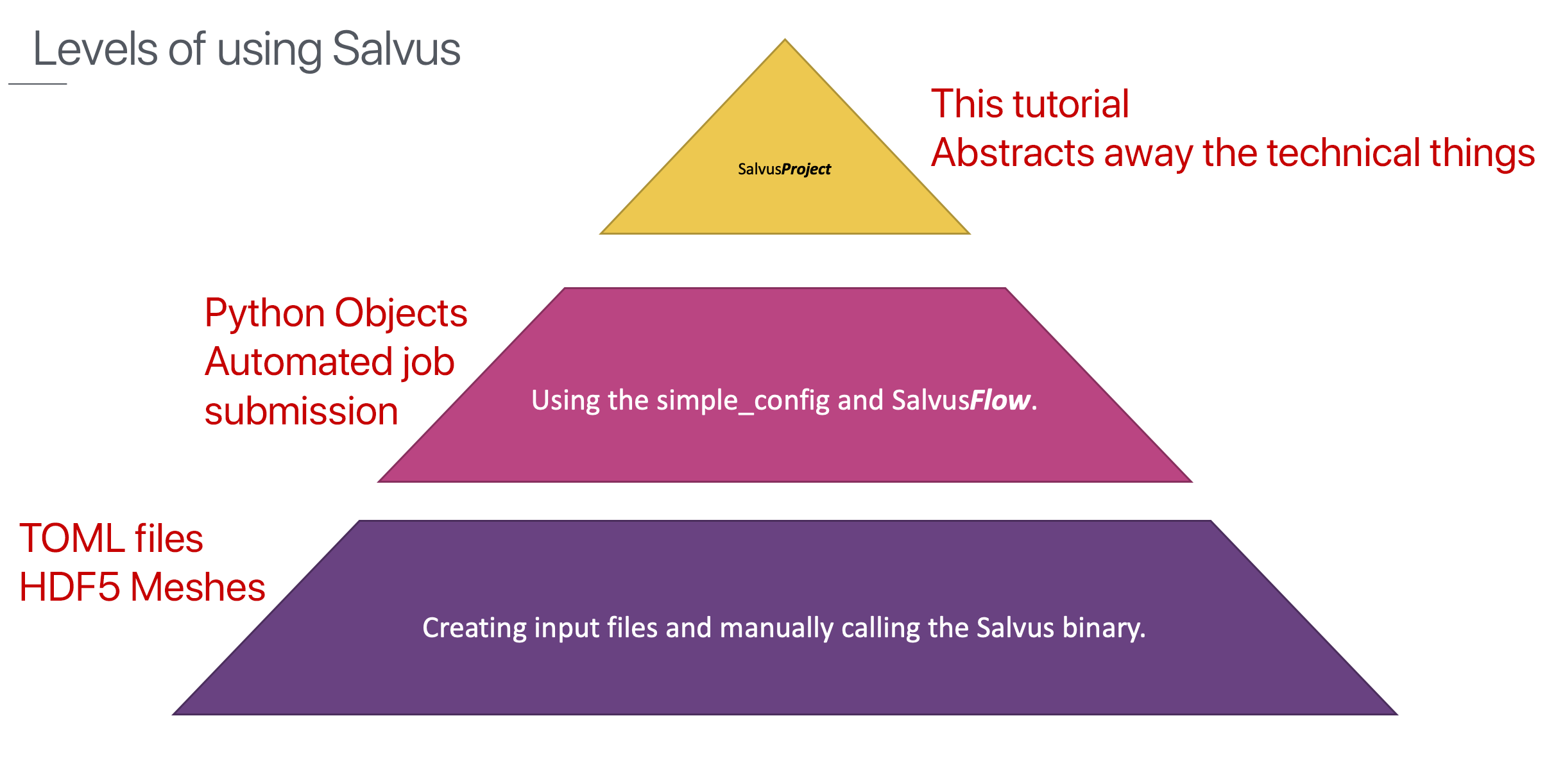
While we use Python to interact with it, you'll notice that very little actual coding is going on. Instead most command can be seen as descriptions of what one wants to do. For advanced use cases it is still possible to code almost every aspect of it. This approach results in a highly automated but also highly flexible way of doing all kinds of waveform simulations and inversions.

It is of course not realistic to fully understand everything we'll present in the next three hours if this is the first time you are seeing it. We also don't have the time to allow for a lot of interactivity.

Instead we hope to demonstrate how to use Salvus to perform waveform simulations and inversions and that you get a feeling for what it can do and the general flow of things. Additionally we try to make it clear where one would have to deviate from this tutorial to tackle other problems.

While we encourage that you follow along, almost everything can also be learned by just watching and maybe asking a few questions.

This tutorial is a full end-to-end program were we go from essentially nothing to an updated model of Earth's structure that better fits the data compared to the starting model. It includes all steps from problem setup, data acquisition and quality control over simulation setup, window picking, and misfit computation to adjoint source derivation and gradients all the way to solving a non-linear optimization problem using a trust-region L-BFGS algorithm.

It is important to realize that Salvus is highly flexible and everything can be modified by you to exactly suit your use case. This includes but is not limited to things like the choice of observed data, starting model, processing functions, misfit functionals, and regularization techniques. In addition most things in this tutorial that are not specific to seismology directly translate to FWI on other domains with Salvus. Examples include seismic exploration as well as medical imaging.

The tutorial is split into 4 parts, each one building on the previous parts:

To start we explain how to choose the inversion domain, how to set up a Salvus project and how to acquire, quality control, and process data.

Once the data side has been dealt with we move towards replicating the data synthetically with waveform simulations.

We have a first look to see how well simulations through the initial model fit the observed data by picking windows. Computing misfits and adjoint sources it the next natural step.

The last part ties everything together and will iteratively update the model and optimize it so it better fits the data with respect to the misfit measurements in the chosen windows.