This documentation is not for the latest stable Salvus version.
The quality of one's starting model has a profound impact on the quality of a subsequent inversion. This is one of the primary steps where we can leverage our prior knowledge of the problem to steer an inversion in the direction we want.
The initial model we want to construct should consist of a 2-D cross section of the shallow subsurface. In general, we want this model to be a smooth representation of the subsurface with material properties which reflect the dominant media within the area of interest.
Given that this process involves using one's prior knowledge of the field, this procedure of generating the starting model can vary greatly from project to project. However, there are some general guidelines one can use to create such an initial model.
A useful approach for constructing an initial model of the subsurface is to apply multi-channel analysis of surface waves (MASW) to construct a 1D model of the subsurface. While Salvus does not currently come bundled with a MASW inversion framework, there are a number of open source tools which are capable of constructing such a starting model:
| Software | Language |
|---|---|
| Geopsy | Graphical User Interface |
| swprocess and swprepost | Python |
| MASWaves | Matlab |
| BayHunter | Python |
When performing field surveys for a particular site, there are often auxiliary sources of information which we can use to constrain our starting model. Some common examples include:
- Standard penetration test (SPT)
- Cone penetration test (CPT)
- Auger or core samples
- Past geotechnical or geophysical surveys conducted in the area
The following approximate S-wave velocity depth profile was obtained using MASW for a single shot position:
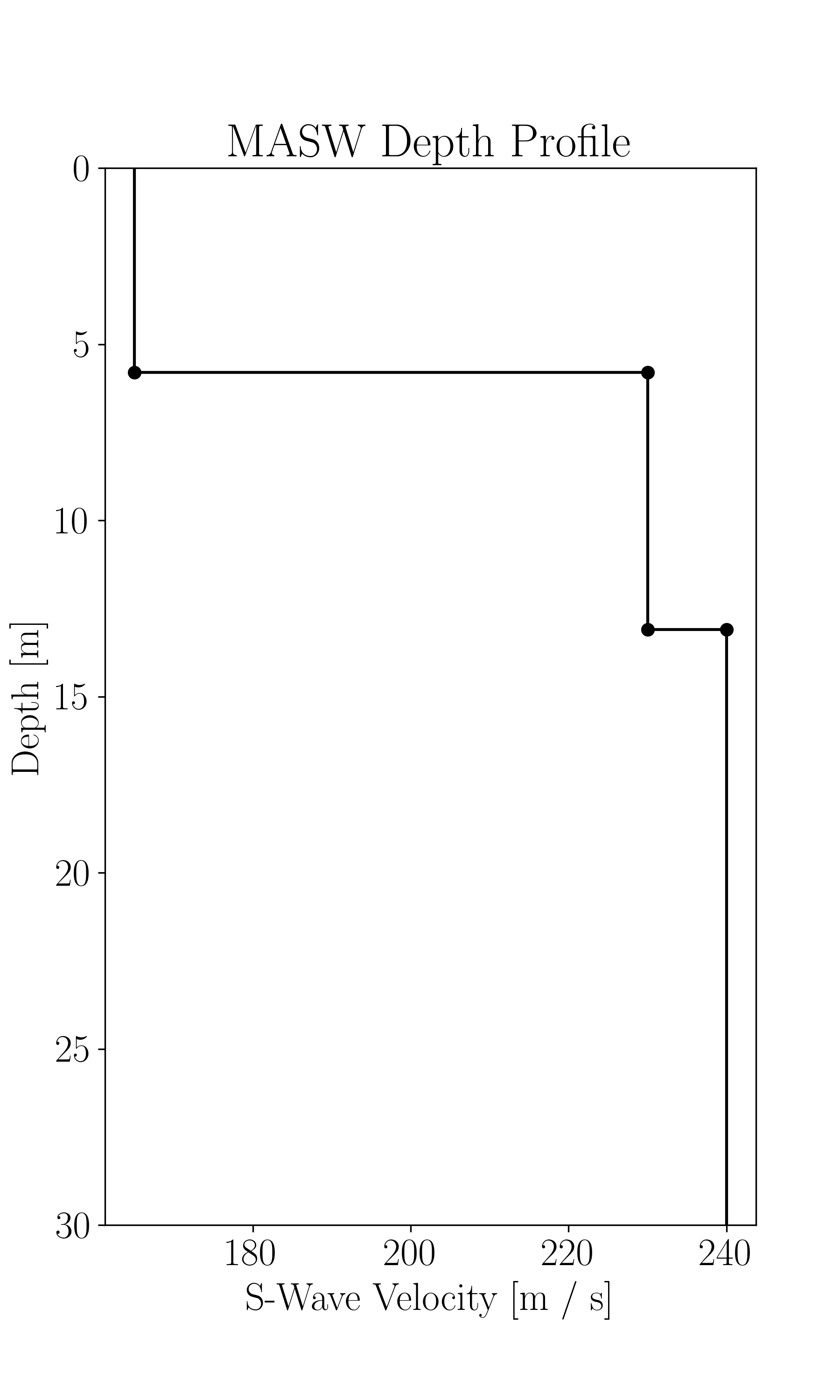
This depth profile will serve as a starting point for generating the initial model used within the FWI workflow.
As usual, let's import a few useful packages as well as open the SalvusProject.
import os

SALVUS_FLOW_SITE_NAME = os.environ.get("SITE_NAME", "local")
PROJECT_DIR = "project"import numpy as np
import xarray as xr
from scipy.ndimage import gaussian_filter1d
import salvus.namespace as snp = sn.Project(PROJECT_DIR)
In order to import the starting model into Salvus, let's create a 2-D Xarray which represents the material properties for the cross section of the subsurface. First, let's create a mask which describes which material property should be assigned to a specific depth interval.
# Define the size of the model to be slightly larger than the domain
buffer = 0.05 * (p.domain.bounds.hc["x"][1] - p.domain.bounds.hc["x"][0]) / 2
nx, ny = 820, 300
x = np.linspace(
    p.domain.bounds.hc["x"][0] - buffer,
    p.domain.bounds.hc["x"][1] + buffer,
    nx,
)
y = np.linspace(
    p.domain.bounds.vc["y"][0] - buffer,
    p.domain.bounds.vc["y"][1] + buffer,
    ny,
)
xx, yy = np.meshgrid(x, y, indexing="ij")

# Approximate 1D model extracted from MASW
model_1D = {
    "depth": np.array([5.8, 13.1, 30.0]),
    "VP": np.array([1600.0, 1750.0, 1800.0]),
    "RHO": np.ones(3) * 2000.0,
    "VS": np.array([165.0, 230.0, 240.0]),
}

# Get an array of which indices correspond to which depth
depths = np.linspace(-y.min(), -y.max(), ny)
depth_inds = np.zeros(ny, dtype=int)
for i in range(len(model_1D["depth"])):
    # For the first layer, just get the values above the first depth
    if i == 0:
        mask = depths <= model_1D["depth"][0]
    # For the last layer, just get the values below the last depth
    elif i == len(model_1D["depth"]) - 1:
        mask = depths > model_1D["depth"][i - 1]
    else:
        mask = (depths > model_1D["depth"][i - 1]) & (
            depths <= model_1D["depth"][i]
        )

    depth_inds[mask] = i
Next, we can use this 1D representation to construct a series of smooth 1D profiles which can then be extruded into 2-D. The reason that we want to use a smooth representation of the material properties here is that there will inevitably be some lateral variability within the material parameters (ie. the material interfaces are likely not perfectly flat). Enforcing a distinct discontinuity at a given location may cause the inversion to converge to a local minimum.
# Create 2-D array of material properties
model_2D = {}
for field in ["VP", "RHO", "VS"]:
    # Create a single depth profile in 1-D
    sharp_1D = np.zeros(ny)
    for i, value in enumerate(model_1D[field]):
        sharp_1D[depth_inds == i] = value

    # Smooth the 1-D model using a gaussian filter
    smooth_1D = gaussian_filter1d(sharp_1D, 10, mode="nearest")

    # Extrude the 1D model to 2-D
    model_2D[field] = (["x", "y"], np.broadcast_to(smooth_1D, [nx, ny]))

# Create an Xarray dataset from the data
ds = xr.Dataset(
    data_vars=model_2D,
    coords={"x": x, "y": y},
)

ds.VP.T.plot(figsize=(10, 6))
<matplotlib.collections.QuadMesh at 0x7f3d022beb90>

Let's now add the material model containing the
VP, RHO, and VS to the SalvusProject. This dataset can first be added to the project as a volume model.model = sn.model.volume.cartesian.GenericModel(name="volume", data=ds)
p.add_to_project(model, overwrite=True)Finally, we can add a new
SimulationConfiguration for this volume model. A few things to note regarding this SimulationConfiguration:max_frequency_in_hertzshould reflect the maximum frequencies which are contained within the source being used. If you aren't sure yet at this stage what your source signature looks like, a good starting point can be to look at the power spectrum for a single trace to see what its dominant frequencies are (see the previous tutorial for an example).tensor_ordercan be chosen as either1,2,4, or7. This controls the number of nodes per element with a higher tensor order resulting in a greater number of nodes per element. Using more nodes per element allows for smoother transitions in material properties throughout the mesh. While using a higher tensor order can increase the file size of the mesh substantially, using higher tensor order meshes does not increase the computational cost of the subsequent wave simulations (apart adding a bit of overhead for reading in the larger mesh from disk) since the number of elements is unaffected.
p.add_to_project(
    sn.SimulationConfiguration(
        name="volumetric_model",
        max_frequency_in_hertz=100.0,
        elements_per_wavelength=1.0,
        tensor_order=2,
        model_configuration=sn.ModelConfiguration(
            background_model=sn.model.background.from_volume_model(
                model=model
            ),
            volume_models=["volume"],
        ),
        event_configuration=sn.EventConfiguration(
            wavelet=sn.simple_config.stf.Ricker(center_frequency=50.0),
            waveform_simulation_configuration=sn.WaveformSimulationConfiguration(
                end_time_in_seconds=0.6
            ),
        ),
    ),
    overwrite=True,
)

p.viz.nb.simulation_setup(
    simulation_configuration="volumetric_model", events=p.events.list()
)
[2024-03-15 10:16:53,352] INFO: Creating mesh. Hang on.

<salvus.flow.simple_config.simulation.waveform.Waveform object at 0x7f3d01546790>
Now that we have an initial model of the subsurface, we can continue with performing a 3D-to-2D conversion on the observed data.

PAGE CONTENTS