Near Surface Waveform Simulations and Data Processing

Many conventional techniques in near surface geophysics such as multi-channel analysis of surface waves (MASW) rely on reconstructing a series of 1D profiles which are subsequently aggregated into a single 2D image. While such methods may be able to resolve large-scale features in the shallow subsurface, they often lack lateral resolution.

The following is an example of full waveform modeling to investigate the near surface. The red marker represents the shot location of an impulsive seismic source (eg. a hammer blow or similar) while the blue markers represent the locations of the receivers. In this example, the subsurface consists of three distinct geological layers which are separated by the beige interfaces.

This tutorial assumes a certain familiarity with Salvus. If you've never used it before, please have a look at our other tutorials.

For this tutorial we'll use SalvusProject, the highest level interface to Salvus.

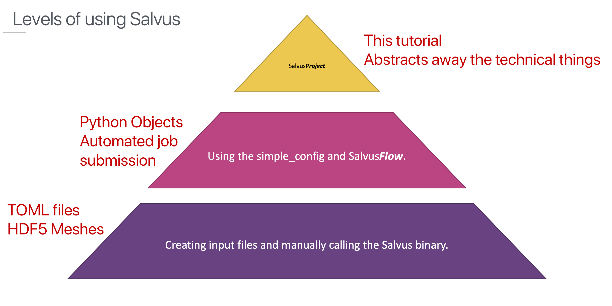
While we use Python to interact with SalvusProject, you'll notice that very little actual coding is going on. Instead most commands can be seen as descriptions of what one wants to do. For advanced use cases it is still possible to code almost every aspect of it. This approach results in a highly automated but also highly flexible way of doing all kinds of waveform simulations and inversions.

This tutorial is split into the following sections:

To start, we go through the process of importing external data into SalvusProject. While this tutorial imports a series of .segy datasets, the procedure is very general and can be easily adapted to work with other file types.

Next, a starting model is constructed based on a priori data of the field site.

Once the initial model has been defined, processing is applied to the observed data (which is inherently 3-D) to make the data appear more "2-D-like". While Salvus can simulate in both 2-D and 3-D, 2-D can lead to considerable computational savings for setups where the variations of the material properties in the out-of-plane direction are small.