Mondaic - Full Waveform Solutions

This tutorial is presented as Python code running inside a Jupyter Notebook, the recommended way to use Salvus. To run it yourself you can copy/type each individual cell or directly download the full notebook, including all required files.

Download Jupyter Notebook [52.09 MB]

The observed data has, of course, been recorded within a 3-D medium. In the interest of computational efficiency, it is desirable to run simulations in 2-D. However, there are inherent differences between data collected within a fully 3-D versus 2-D domain. In this tutorial, we will go through the process of performing this 3D-to-2D conversion in addition to providing a conceptual overview of what this process looks to accomplish.

Please note that the underlying theory for this 3D-to-2D conversion can be found within the following two publications and the references therein:

Forbriger, T., L. Groos, M. Schäfer (2014). Line-source simulation for shallow-seismic data. Part 1: theoretical background. Geophysical Journal International, 198(3), 1387-1404. https://dx.doi.org/10.1093/gji/ggu199

Schäfer, T., M., L. Groos, T. Forbriger, T. Bohlen (2014). Line-source simulation for shallow-seismic data. Part 2: full-waveform inversion — a synthetic 2-D case study. Geophysical Journal International, 198(3), 1405-1418. https://dx.doi.org/10.1093/gji/ggu171

A 2-D simulation implicitly assumes that the effects in the out-of-plane direction are uniform. This effectively means that an equivalent 3-D simulation would require us to extrude everything in the 2-D domain in the out-of-plane direction.

A point source in 2-D generates a circular wavefront which propagates away from the source position:

Given our previous definition of going from a 2-D setup to a 3-D equivalent, this would mean that the wavefront should be extruded in the out-of-plane direction as well. This would look something like the following:

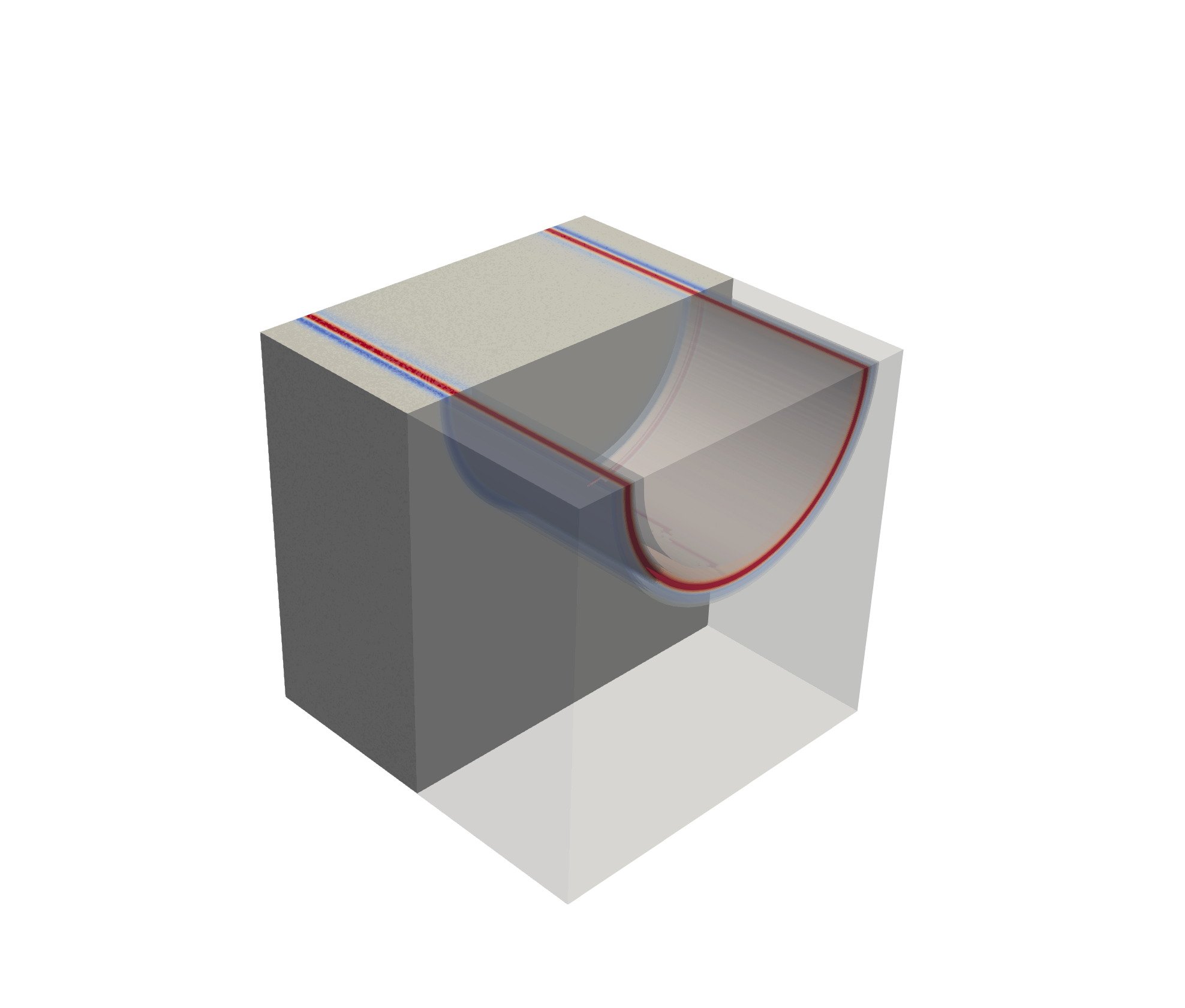
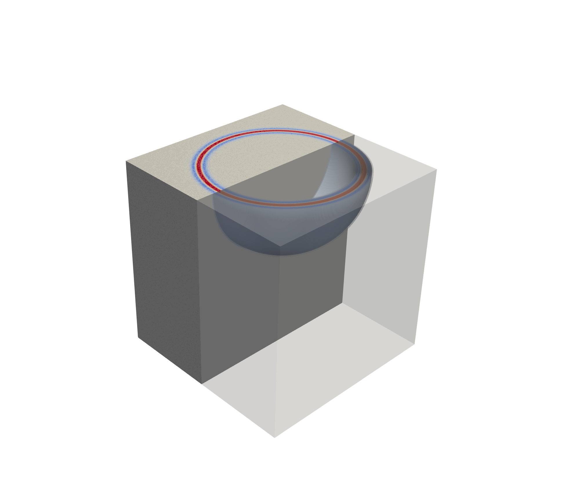
If we consider a fully 3-D simulation, an idealized point source emits energy equally in all directions. Thus, a spherical wavefront is, in fact, generated:

Thus, we want to have some conversion to allow for our observed data, which was created using a spherical wavefront, to appear as though it were generated using such a cylindrical wavefront. This process is often referred to as a point source to line source conversion given that such a cylindrical wavefront can be approximated using a line source, which is oriented in the out-of-plane direction.

Let's start by importing a few Python packages along with the SalvusProject:

Copy

PROJECT_DIR = "project"

Copy

import matplotlib.pyplot as plt
import numpy as np

import salvus.namespace as sn
from salvus.modules.near_surface.processing import convert_point_to_line_source

Copy

p = sn.Project(path=PROJECT_DIR)

To apply a processing function to data which is already within SalvusProject, we apply two separate steps:

Define a callback function which accepts an obspy.Stream containing the information about the traces we want to apply the processing to along with the Salvus source/receiver objects.
A ProcessingConfiguration which specifies which data we want to apply the processing to in addition to the callback function itself.

Here we will use the hybrid transform discussed in the two papers referenced in the introduction of this notebook. This transformation involves applying two different transformations to the data depending on the receiver's offset relative to the source:

The single-velocity method is used for near offsets
The direct-wave method is used for further offsets

There are two additional parameters which need to be defined for this transform type, namely:

velocity_m_s: Reference velocity for the medium. While this theoretically assumes that the medium consists of a homogeneous full-space, using an average of the velocities within the top portion of the medium generally seems to yield adequate results.
hybrid_transformation_transition_zone: The distances within which each transform should be applied. In this case, hybrid_transformation_transition_zone should be a list of distances where the the single-velocity method is applied to the receivers below the first value in the transition zone while the direct-wave method is applied to the receivers beyond the second value in the transition zone.

First, let's get the velocity_m_s by averaging the "VS" from our initial model over the first ~5.0 m depth of the model. We start by getting the mesh of the starting model.

Copy

m = p.simulations.get_mesh("volumetric_model")

Next, we can create a mask of all of the elements which are above a depth of 5.0 m and then take the average of the "VS" over this depth range.

Copy

depth = -5.0
field = "VS"

# Create a mask of the elements which are above a depth of 5.0 m
mask = m.get_element_centroid()[:, 1] > -5.0

# Take the mean of the "VS" for the masked out elements
velocity_m_s = np.mean(m.elemental_fields[field][mask, :])

print(
    f"The average `{field}` above {np.abs(depth)} m is {np.round(velocity_m_s, 1)} m/s"
)

The average `VS` above 5.0 m is 166.9 m/s

The choice of the transition zone is somewhat subjective. Here we will treat the "near offsets" as being less than 5.0 m offset relative to the source while "far offsets" will be treated as being at greater than 10.0 m offsets.

Next, let's define the callback function.

Copy

def processing_3d_to_2d(st, sources, receiver):
    st = convert_point_to_line_source(
        st=st,
        source_coordinates=np.array(sources[0].location),
        receiver_coordinates=np.array(receiver.location),
        transform_type="hybrid",
        velocity_m_s=velocity_m_s,
        hybrid_transformation_transition_zone=[5.1, 10.1],
    )

    return st

This can then be passed into a new ProcessingConfiguration which we will use to apply the 3D-to-2D conversion onto the EXTERNAL_DATA:survey_data, which was added during the first tutorial of this series.

Copy

p.add_to_project(
    sn.processing.ProcessingConfiguration(
        name="calibrated_3d_to_2d",
        data_source_name="EXTERNAL_DATA:survey_data",
        processing_function=processing_3d_to_2d,
    ),
    overwrite=True,
)

Finally, let's compare the waveforms from before and after applying the 3D-to-2D conversion.

Copy

p.viz.shotgather(
    data=["EXTERNAL_DATA:survey_data", "PROCESSED_DATA:calibrated_3d_to_2d"],
    event=p.events.list()[0],
    receiver_field="velocity",
    component="X",
)

<Axes: title={'center': 'Event: 00 | field: velocity | component: X'}, xlabel='Receiver Index', ylabel='Time [s]'>

Note that this conversion has not only changed the ampltidues of the signal, but also the phase. This can be nicely visualized when plotting individual traces:

Copy

p.viz.nb.waveforms(
    data=["EXTERNAL_DATA:survey_data", "PROCESSED_DATA:calibrated_3d_to_2d"],
    receiver_field="velocity",
)

This has applied a fairly significant correction to the 3-D data to make it more "2-D-like". Note that since we've only provided a single component of the velocity data at the start of the project, only a single component is plotted within the waveforms.

Part 2 - Starting Model

Semi-analytic test - Acoustic

Site Map Contact Us

Impressum

Academic License Agreement

Credits

PAGE CONTENTS