Mondaic - Full Waveform Solutions

This tutorial is presented as Python code running inside a Jupyter Notebook, the recommended way to use Salvus. To run it yourself you can copy/type each individual cell or directly download the full notebook, including all required files.

Download Jupyter Notebook [21.47 MB]

The first part of the continental scale full waveform inversion tutorial explains how to set up the spatial domain and how to acquire observed data for it.

Copy

MIN_PERIOD = 70.0
MAX_PERIOD = 120.0
SIMULATION_TIME_IN_SECONDS = 1200.0
SALVUS_FLOW_SITE_NAME = "local"
RANKS_PER_JOB = 8
PROJECT_DIR = "project_dir_central_europe"

period_band_name = f"{int(MIN_PERIOD)}_{int(MAX_PERIOD)}_seconds"

Copy

import pathlib
from salvus import namespace as sn

The first crucial choice is the choice of spatial domain, i.e. which region you want to invert for. A hard constraint in FWI is that sources and receivers must both be part of the domain - this means that teleseismic events are not usable aside from inversions for the full globe.

In most cases you will already know which region you want to invert it. Nonetheless it is useful to have a look at seismicity and station maps. Oftentimes it is worthwhile to extend the domain to include extra sources and receivers, because FWI in seismology is fundamentally limited by the available data and more is always better.

Not all earthquakes can be used. Two main restrictions limit the acceptable magnitude range, both are a function of the domain size as well as the period range one is interested in.

Must be big enough to be measurable across the whole domain in the frequency range of interest. Small earthquakes additionally don't excite a lot of low frequency surface wave energy which further limits their use especially in the initial, long-period iterations of an inversion. This is dependent on the sites' instrumentations and noise levels and no general rule can be given and it has to be figured out by trial and error. Most studies set the minimum moment magnitude to a value between 4 and 5.

The earthquakes must be small enough so that they can be reasonably approximated by a point source. It is okay if the source mechanisms captures some of the finite fault nature. The rupture length of the earthquake should be significantly smaller than the smallest wavelength one is interested in, which is especially important for receivers close to the fault.

This is a deep topic and strongly dependent on the region and type of fault but the following figure empirically relates fault length to moment magnitude. There are no hard rules but between moment magnitudes from 6 to 7.5 the fault length approximately ranges from 10 to 100 km and depending on the chosen region and frequency range the maximum magnitude one uses for a continental scale full waveform dimension should be in that range.

Common moment magnitude vs fault length relations, constants taken from Leonard, M. (2014). Self-Consistent Earthquake Fault-Scaling Relations: Update and Extension to Stable Continental Strike-Slip Faults. Bulletin of the Seismological Society of America, 104(6), 2953–2965. doi:10.1785/0120140087

For this tutorial we will study central Europe. The following image shows the seismicity of Europe and the approximate domain of interest.

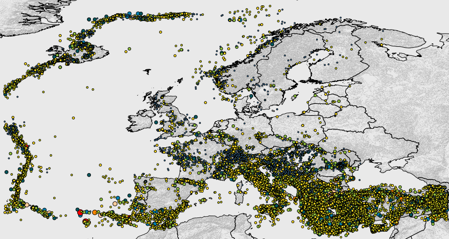
Screenshot from the EFEHR Hazard Map Portal, CC BY-SA 3.0 (unported).

SalvusProject has a number of different domains that are suitable for different use cases.

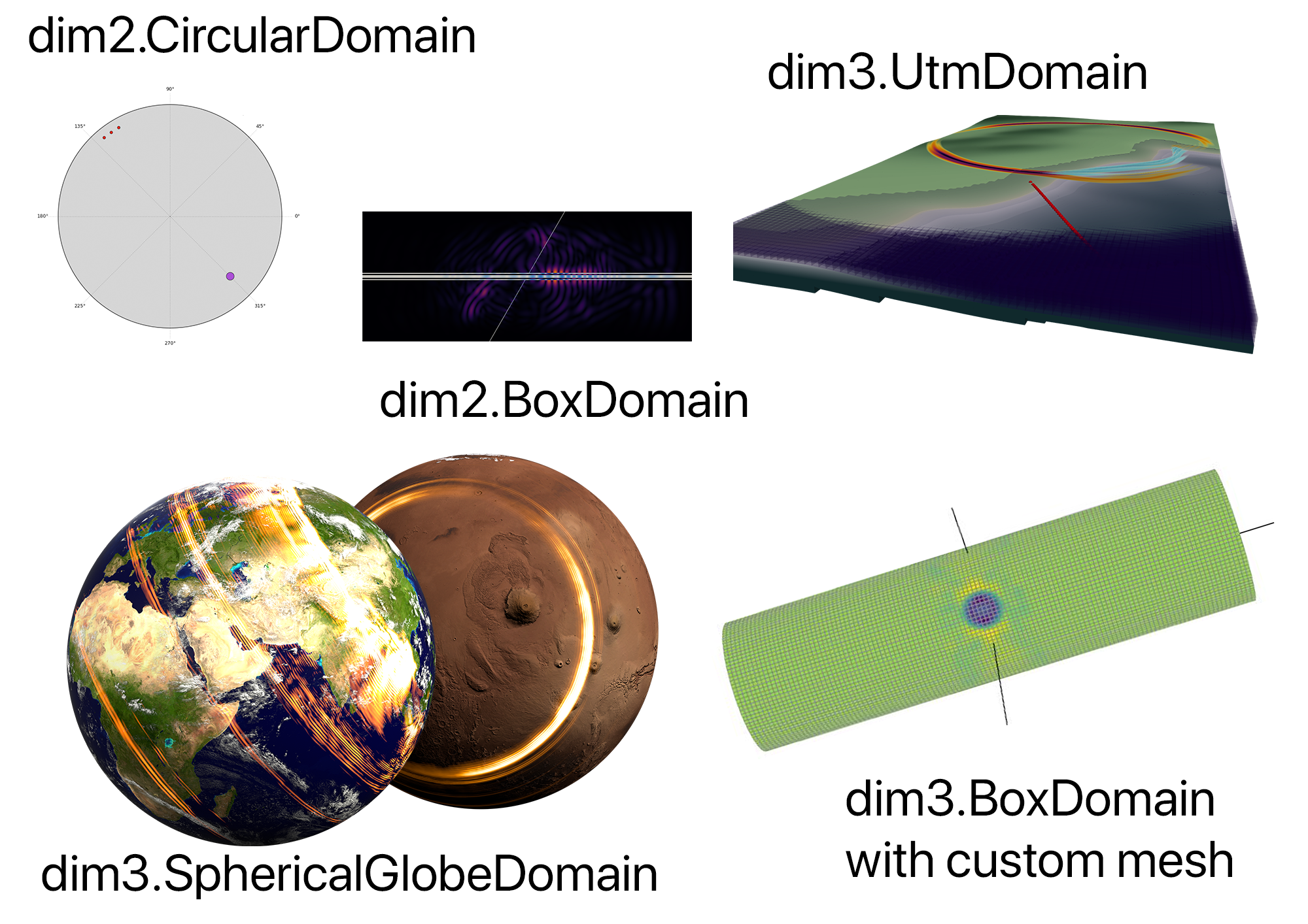
In Salvus we can describe this as a spherical chunk on the surface of the Earth. So let's start by defining this domain and center a new Project around it. Domain objects can be visualized so it is easy to try a few values until the desired result is achieved. This will be the inversion domain so the goal here is to get as close to the desired region as possible as it cannot be changed after a project has been created. The map projections between the above image and the domain plot are different but they show a very similar region.

Copy

lat_center, lon_center = 48.0, 10.0
lat_extent, lon_extent = 25.0, 25.0

domain = sn.domain.dim3.SphericalChunkDomain(
    lat_center=lat_center,
    lat_extent=lat_extent,
    lon_center=lon_center,
    lon_extent=lon_extent,
    radius_in_meter=6371e3,
)

domain.plot()

That looks close enough to the desired region so we'll now create a new project from it. A project is a persistent structure on disc that enables to run simulations and whole inversions with Salvus in a declarative manner.

Copy

p = sn.Project.from_domain(
    path=pathlib.Path(PROJECT_DIR), domain=domain, load_if_exists=True
)

Data downloading can be very time consuming. Thus this tutorial contains an existing project where the data has already been downloaded. Thus many of the following cells will not do anything.

Before we can start to simulate or even invert we need to acquire some data. In many realistic scenarios you might already have this - here we'll utilize a few utility functions coming with Salvus that first add a number of earthquakes to the project and then downloads waveform and station information for these events.

In case you already have the data it is best to convert the waveform as well as the station and earthquake data to ASDF files. The most useful layout it to have one ASDF file per event. The data can already be preprocessed or the processing can be applied on-the-fly by Salvus project.

To ensure reproducibility, you find pre-selected 11 events and accompanying waveform data in the downloaded material. Alternatively, Salvus can fully automatically acquire earthquake information by querying the GCMT catalog and waveform and station information by utilizing the FDSN web services for the target region. You may skip the next cell if you want to use the automated downloader instead.

Copy

if not p.events.list():
    for file in sorted(pathlib.Path("data").glob("*.h5")):
        print(f"Adding external data from `{file}`")
        p.actions.seismology.add_asdf_file(
            filename=file,
            data_name="raw_data",
            receiver_fields=["displacement"],
        )

Adding external data from `data/event_CRETE_GREECE_Mag_6.15_2015-04-16-18-07.h5`
Adding external data from `data/event_ICELAND_REGION_Mag_5.75_2020-06-20-19-26.h5`
Adding external data from `data/event_STRAIT_OF_GIBRALTAR_Mag_6.38_2016-01-25-04-22.h5`

SalvusProject can add events from a specially prepared CSV catalog file. In this case it will choose an optimal subset of events and add them to the domain. It is optimal in the sense that it successively chooses new events by always choosing the one event that has the largest minimum distance to the next closest existing event.

Mondaic offers the preprocessed CSV files for download (click here).

In case you skipped the previous cells, there are still no events in our project, and the following cell will create a list of earthquakes from the database.

Copy

if not p.events.list():
    p += p.actions.seismology.get_events_from_csv_catalog_file(
        filename="./data/gcmt_catalog.csv.bz2",
        max_count=30,
        min_moment_magnitude=5.75,
        max_moment_magnitude=6.5,
        min_distance_in_meters=500e3,
        min_year=2010,
        max_year=2020,
        random_seed=123456,
    )

Once we are satisfied with the chosen events we can call a utility function to download publicly available waveform data as well as station meta information.

Copy

for event in p.events.list():
    if p.waveforms.has_data("EXTERNAL_DATA:raw_data", event=event):
        continue

    p.actions.seismology.download_data_for_event(
        data_name="raw_data",
        event=event,
        # If you leave this empty all providers will be queried.
        download_providers=["IRIS"],
        add_receivers_to_project_event=True,
        receiver_fields=["displacement"],
        seconds_before_event=240.0,
        seconds_after_event=1.2 * SIMULATION_TIME_IN_SECONDS,
    )

Copy

p.viz.nb.domain()

We are doing an inversion with real data here and it is important to make sure the data is actually suitable to be inverted for. It thus always a good idea to have a look at some data before continuing. SalvusProject has a few convenience visualization routines to aid in that task but you are of course free to use any other tool you see fit.

Copy

p.viz.nb.waveforms(
    data="EXTERNAL_DATA:raw_data", receiver_field="displacement"
)

There should be very visible wave trains arriving at most stations - otherwise something went wrong. The raw data can of course also not be used directly for a full waveform inversion.

It is okay if some stations have not recorded the data well or have clipping or other quality issues - later stages in the inversion process will filter these out. But the majority of stations should have recorded the earthquakes and it should be clearly visible in the seismograms.

You might have noticed the EXTERNAL_DATA:raw_data data name. SalvusProject refers to waveform data by data type (or namespace if you will) and name within that data type. Everything before the colon is the data type, everything after the name. If no data type is given it will default to SYNTHETIC_DATA. SalvusProject distinguishes three data types:

SYNTHETIC_DATA: Synthetically computed waveforms. These are always computed within the project structure.
EXTERNAL_DATA: Observed or externally computed waveform data.
PROCESSED_DATA: Any processed data. The data can originate from synthetic, external or even other processed data but a function sits in between that processed the data in some fashion.

This naturally leads us into data processing which is always necessary in seismology. In this case we'll use it to remove the instrument response and to filter the data to frequencies we will actually invert for.

There are many choices to be made here and it might very well be that you will have to write you own processing function to account for specifics of your particular problem set. We'll use a helper function in SalvusProject' tools to generate such a processing function. In case you have non-standard processing needs you can also replace it with your own custom function.

The function will first decimate the data a bit to speed up subsequent operations, then remove the instrument response and finally filter the data in the chosen frequency range. Additionally it will rotate it to the ZNE coordinate system in case there is data with arbitrary orientations (oftentimes the case for GSN stations).

An important choice here is the period band which we will set from 70 to 120 seconds. This is very long period and we expect only to match the surface waves but it should have a good initial data fit and enable a few cheap initial iterations.

This function processes data in a fashion that is compatible with Salvus' FilteredHeaviside source time function. This will become crucial at later stages because it saves us from having to process the synthetics (and account for that in the adjoint source computation).

Copy

from salvus.project.tools.processing.seismology import (
    get_remove_response_and_bandpass_filter_processing_function,
)

processing_function = (
    get_remove_response_and_bandpass_filter_processing_function(
        min_frequency_in_hertz=1.0 / MAX_PERIOD,
        max_frequency_in_hertz=1.0 / MIN_PERIOD,
        highpass_corners=3,
        lowpass_corners=3,
        zerophase=False,
    )
)

Once this function has been defined it can be added to a project as a so called processing configuration. A processing configuration has a name to identify it, a data source name where the data is taken from before the processing is applied as well as the just created function.

The goal here is again that the waveforms are clearly visible and the signal to noise ratio is good. This will not be the case for all stations but for a large fraction is should. You do not have to manually exclude waveforms - the fit to the data and especially the later window selection are the final authority and in most cases this work very well.

Copy

p.add_to_project(
    sn.processing.seismology.SeismologyProcessingConfiguration(
        name=period_band_name,
        data_source_name="EXTERNAL_DATA:raw_data",
        processing_function=processing_function,
    ),
    overwrite=True,
)

p.viz.nb.waveforms(
    [f"PROCESSED_DATA:{period_band_name}"],
    receiver_field="displacement",
)