This documentation is not for the latest stable Salvus version.
In this tutorial we'll set up, from scratch, a 3-D spherical domain for the region surrounding Australia. This domain will include a 3-D crustal and mantle model, taken from AusREM, as well as 3-D surface and Moho topography. After our model and simulations are set up, we'll fire them off to a remote site (if available) in order to run simulations accurate to a minimum period of 40 seconds. We'll then gather the data from the remote site and apply some basic processing functions to some observed, as well as our synthetic, data. All right -- let's get started!
# This notebook will use this variable to determine which
# remote site to run on.
import os
import pathlib
import time

from salvus import namespace as snSALVUS_FLOW_SITE_NAME = os.environ.get("SITE_NAME", "local")
PROJECT_DIR = "project"We start by initializeing a small domain centered on Australia, and download real data via ObsPy for a few stations from the
IU global network. These are high quality stations which will be perfect for a comparison to our synthetic data.If the project already exist on disk, the cell below allows us to simply load the project.
# Define a spherical chunk domain.
lat_c, lon_c = -27.5, 135
lat_e, lon_e = 25.5, 42.0
d = sn.domain.dim3.SphericalChunkDomain(
    lat_center=lat_c,
    lat_extent=lat_e,
    lon_center=lon_c,
    lon_extent=lon_e,
    radius_in_meter=6371e3,
)

p = sn.Project.from_domain(
    path=PROJECT_DIR,
    domain=d,
    load_if_exists=True,
)
# Add an event
e = sn.Event(
    sources=sn.simple_config.source.seismology.parse(
        "./data/event.txt", dimensions=3
    ),
    receivers=[],
)if e.event_name not in p.events.list():
p.add_to_project(e)
p.actions.seismology.download_data_for_event(
data_name="raw_recording",
event=p.events.list()[0],
add_receivers_to_project_event=True,
receiver_fields=["velocity"],
seconds_before_event=300.0,
seconds_after_event=1800.0,
network="IU",
download_providers=["IRIS"],
)In previous tutorials we outlined the difference between background and volumetric models, and until now have only considered background models. Here we'll foray into the use of volumetric models as well, and we'll specifically choose a different model for both the crust and the mantle. In the tutorial folder you should see two NetCDF (
.nc) files entitled ausrem_crust.nc and ausrem_mantle.nc. The name of these models are relatively self descriptive: they are modified version of the AusREM (Australian Seismological Reference Model) crust and mantle models respectively. The format that they are stored in is governed by the CF conventions, which is a commonly used format for storing geoscientific data.Since we're focussed here on Australia we'll shift back to AusREM for now. In a seismological context, we can restrict the interpolation of models to specific regions, such as the crust or mantle. Also, in many cases we want to apply a taper to the volumetric models so that they will smoothly blend into the background model. To accomplish this, the seismological model API allows us to optionally specify a
taper_in_degrees parameter. Ok, now let's add the crustal model to the project...p.add_to_project(
sn.model.volume.seismology.CrustalModel(
name="ausrem_crust",
data="./data/ausrem_crust.nc",
taper_in_degrees=5.0,
)
)...and now the mantle model...
p.add_to_project(
    sn.model.volume.seismology.MantleModel(
        name="ausrem_mantle",
        data="./data/ausrem_mantle.nc",
        taper_in_degrees=5.0,
    )
)
...and now finally let's create a complete model configuration using anisotropic PREM as a background model.
mc = sn.ModelConfiguration(
    background_model="prem_ani_one_crust",
    volume_models=["ausrem_crust", "ausrem_mantle"],
)Surface and Moho topography can be added in a similar fashion to those on Cartesian domains.
These files contain filtered versions of global surface and moho topography.
p.add_to_project(
    sn.topography.spherical.SurfaceTopography(
        name="topo_surface",
        data="./data/topography_wgs84_filtered_512.nc",
        use_symlink=True,
    )
)p.add_to_project(
sn.topography.spherical.MohoTopography(
name="topo_moho",
data="./data/moho_topography_wgs84_filtered.nc",
use_symlink=True,
)
)tc = sn.topography.TopographyConfiguration(
topography_models=["topo_surface", "topo_moho"]
)To finalize our simulation configuration, we first prepare an event configuration to define the time and frequency axes. We'll simulate half an hour of synthetic waveforms, and take as our source time function a Gaussian in moment-rate. In this case we'll set a very short half-duration in seconds to get an almost white spectrum in our synthetic data. We'll use this to motivate the processing functions we later apply.
# end_time_in_seconds should be 1800.0 s!
# We only truncated the time interval for the CI.

ec = sn.EventConfiguration(
    wavelet=sn.simple_config.stf.GaussianRate(half_duration_in_seconds=1.5000),
    waveform_simulation_configuration=sn.WaveformSimulationConfiguration(
        end_time_in_seconds=10.0
    ),
)
As always, we need to also set up some absorbing boundary parameters here. At this point it is fair to ask the question: how do I choose a reference velocity in a domain with a 3-D velocity model, and what even is the reference frequency if my spectrum is white? The answer to both of these questions is that, as always, the performance of the absorbing boundaries is a tunable parameter. In the case of a white spectrum a good rule is to set the reference frequency to the dominant frequency in your observed data.
ab = sn.AbsorbingBoundaryParameters(
    reference_velocity=6000.0,
    number_of_wavelengths=3.5,
    reference_frequency=1 / 40.0,
)We've now got everything we need to set up our simulation configuration object, as we do in the next cell below. Here we'll generate a simulation mesh which ensures that we have at least 1 element per wavelength using a minimum period of 40 seconds, and the using anisotropic PREM as a size function.
# Combine everything into a complete configuration.
p.add_to_project(
    sn.SimulationConfiguration(
        tensor_order=1,
        name="40seconds",
        elements_per_wavelength=1.0,
        min_period_in_seconds=40,
        max_depth_in_meters=1000e3,
        model_configuration=mc,
        topography_configuration=tc,
        event_configuration=ec,
        absorbing_boundaries=ab,
    )
)
We can, as is true with the other domains, visualize our new simulation configuration...
p.viz.nb.simulation_setup("40seconds", events=p.events.list())[2024-03-15 09:34:05,166] INFO: Creating mesh. Hang on.
Interpolating model: ausrem_crust.
Interpolating model: ausrem_mantle.

<salvus.flow.simple_config.simulation.waveform.Waveform object at 0x7f6125495dd0>
... and then go ahead and run our simulation. The time taken to complete will vary significantly depending on the options you've chosen above. For instance, adding both Moho and surface topography decreases the time step by quite a bit due to the relatively small elements in the oceanic crust.
p.simulations.launch(
    ranks_per_job=4,
    site_name=SALVUS_FLOW_SITE_NAME,
    events=p.events.list()[0],
    wall_time_in_seconds_per_job=3600,
    simulation_configuration="40seconds",
)

p.simulations.query(block=True, ping_interval_in_seconds=10.0)
[2024-03-15 09:34:07,446] INFO: Submitting job ... Uploading 1 files... 🚀 Submitted job_2403150934556448_dc1027e62d@local

True
It is usually necessary to process files to be able to compare data to synthetics.
# Import helper function generating suitable processing functions.
from salvus.project.tools.processing.seismology import (
    get_bandpass_filter_processing_function,
    get_remove_response_and_bandpass_filter_processing_function,
)p.add_to_project(
sn.processing.seismology.SeismologyProcessingConfiguration(
name="observed_40_seconds",
data_source_name="EXTERNAL_DATA:raw_recording",
processing_function=get_remove_response_and_bandpass_filter_processing_function(
min_frequency_in_hertz=1.0 / 100.0,
max_frequency_in_hertz=1.0 / 40.0,
highpass_corners=4,
lowpass_corners=4,
),
),
# Useful here to quickly play around.
overwrite=True,
)p.add_to_project(
sn.processing.seismology.SeismologyProcessingConfiguration(
name="synthetic_40_seconds",
data_source_name="40seconds",
processing_function=get_bandpass_filter_processing_function(
min_frequency_in_hertz=1.0 / 100.0,
max_frequency_in_hertz=1.0 / 40.0,
highpass_corners=4,
lowpass_corners=4,
),
),
overwrite=True,
)p.viz.nb.waveforms(
[
"PROCESSED_DATA:observed_40_seconds",
"PROCESSED_DATA:synthetic_40_seconds",
],
receiver_field="velocity",
)
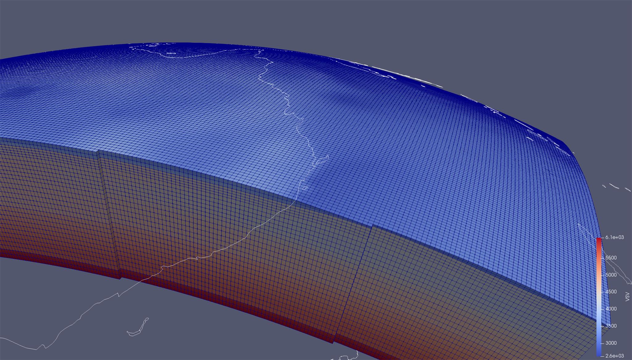
The
.nc files we used in this tutorial are in fact the same convention that is used by the IRIS Earth Model Catalogue (EMC). This means that many of the models stored in the EMC can be downloaded and used
directly in Salvus! Unfortunately, there is no standard parameter set stored in the EMC, and we've found that not all the files actually conform to the required convention. Nevertheless, with some minimal processing, you can have the public library of 3-D Earth models at your disposal to run simulations through. The picture below show a successful attempt at including 3 distinct 3-D Earth models (crust, mantle, cascadia) for a region along the US west coast.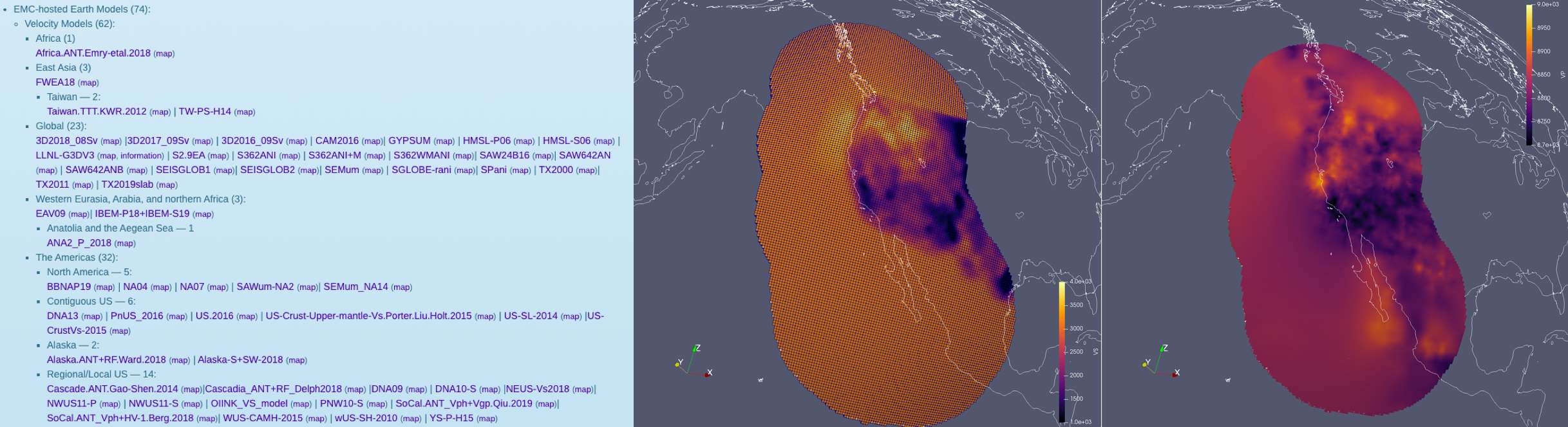
# # Adding the downloaded file as a mantle model.
# p += sn.model.volume.seismology.MantleModel(
#     name="SEMUM", data="./SEMUM_kmps.nc"
# )# # Combine into a model configuration.
# mc1 = sn.model.ModelConfiguration(
# background_model="prem_iso_one_crust", volume_models=["SEMUM"]
# )# # Combine everything into a complete configuration.
# p += sn.SimulationConfiguration(
# tensor_order=1,
# name="40seconds_semum",
# elements_per_wavelength=1.0,
# min_period_in_seconds=40,
# max_depth_in_meters=1000e3,
# model_configuration=mc1,
# topography_configuration=tc,
# event_configuration=ec,
# absorbing_boundaries=ab,
# )# # Visualize the setup.
# p.viz.nb.simulation_setup("40seconds_semum", events=p.events.list())# # Can also open it in Paraview.
# m = p.simulation.get_mesh_filenames("40seconds_semum")["xdmf_filename"]
# # Uncomment the following line on Mac OS
# # !open {m}
PAGE CONTENTS