This documentation is not for the latest stable Salvus version.
The effects of free-surface topography on seismic waveforms are significant, and any local study considering higher-frequency data must take topography into account. In this tutorial we'll explore how to add realistic free-surface topography to a
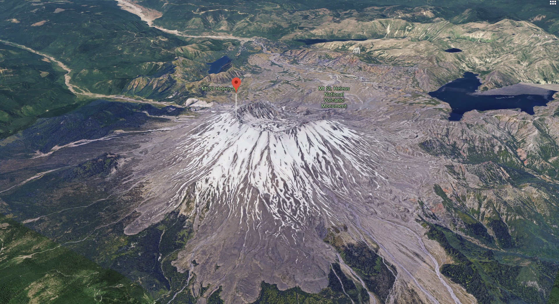
SimulationConfiguration object, and investigate how high-order accurate topography / material interpolation can be used to improve simulation performance. To accomplish this, we'll focus on a real-life use case using the area around Mt. St. Helens in Washington state as an example. Of course please feel free to adapt the geographical area.As always, we'll start by importing the Salvus namespace.
%matplotlib inline
import os
import pathlib
import salvus.namespace as sn# This notebook will use this variable to determine which
# remote site to run on.
SALVUS_FLOW_SITE_NAME = os.environ.get("SITE_NAME", "local")
PROJECT_DIR = "project"There are a number of ways topography can be specified in Salvus. In addition it has two built-in ways to acquire real world digital elevation data at fairly high resolution:
We focus on the first approach for the purpose of this tutorial. At the end there is an appendix to demonstrate how to use data acquired via the AppEEARs web service.
The first step is to define the geographical domain of interest. A convenient way to do this is to use the specialized
UtmDomain.from_spherical_chunk constructor that takes WGS84 coordinates and converts them to an appropriate UTM domain. The UTM zone and coordinates could of course also be specified directly.d = sn.domain.dim3.UtmDomain.from_spherical_chunk(
min_latitude=46.15,
max_latitude=46.30,
min_longitude=-122.28,
max_longitude=-122.12,
)
# Have a look at the domain to make sure it is correct.
d.plot()
# Where to download topography data to.
topo_filename = "data/gmrt_topography.nc"# Now query data from the GMRT web service.
if not pathlib.Path(topo_filename).exists():
d.download_topography_and_bathymetry(
filename=topo_filename,
# The buffer is useful for example when adding sponge layers
# for absorbing boundaries so we recommend to always use it.
buffer_in_degrees=0.1,
resolution="default",
)# Load the data to Salvus compatible SurfaceTopography object. It will resample
# to a regular grid and convert to the UTM coordinates of the domain.
# This will later be added to the Salvus project.
t = sn.topography.cartesian.SurfaceTopography.from_gmrt_file(
name="st_helens_topo",
data=topo_filename,
resample_topo_nx=200,
# If the coordinate conversion is very slow, consider decimating.
decimate_topo_factor=5,
# Smooth if necessary.
gaussian_std_in_meters=0.0,
# Make sure to pass the correct UTM zone.
utm=d.utm,
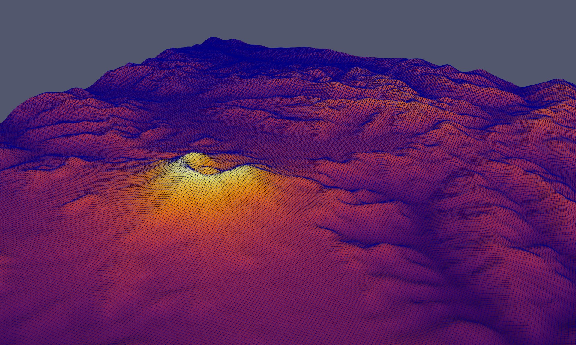
)The interface we just used above to read in topography data is very general and also works for other data formats, and we'll see in a future tutorial how to read in surface, Moho, or discontinuity topography using a similar simplified interface. As is true for the volumetric models used in Salvus, once the topography files are read and processed they are stored as xarray datasets in memory. These datasets are simple to manipulate and visualize, and we can for instance plot the digital elevation model in the notebook by simply plotting the xarray dataset.
t.ds.dem.T.plot(aspect=1, size=7)<matplotlib.collections.QuadMesh at 0x7f44bb853390>

Looks like St. Helens to me!
We can now create/load the project as seen in many other tutorials.
# Uncomment the following line to delete a
# potentially existing project for a fresh start
# !rm -rf project
p = sn.Project.from_domain(path=PROJECT_DIR, domain=d, load_if_exists=True)
Adding the previously downloaded and parsed topography is as simple as adding the
SurfaceTopography object to Salvus:p += tSalvus is now aware of this topography and it can be used for simulations.
p.entities.list("topography_model")['st_helens_topo']
Now we'll add an explosive source and a line of receivers to the project. Here we use the
SideSet source and receiver classes. The functionality of these classes is documented here. Essentially, they help when the actual surface of the domain is non-trivial, as is the case in this example. When these sources and receivers are associated with a mesh, a small optimization problem is solved to ensure that they are placed exactly at the surface of the deformed mesh, plus or minus any offset one might specify. Here we specify the entities in UTM coordinates, place the source 1000 meters below the free surface, and place a line of 50 receivers directly at the free surface.# Src / Rec reference coordinates.
src_x, src_y, src_z = 562700.0, 5112500.0, 4000.0
rec_x, rec_y, rec_z = 564700.0, 5115500.0, 4000.0# Place an explosive source 1000 m below the free surface.
src = sn.simple_config.source.cartesian.SideSetMomentTensorPoint3D(
point=(src_x, src_y, src_z),
direction=(0, 0, 1),
side_set_name="z1",
mxx=1e21,
myy=1e21,
mzz=1e21,
myz=0.0,
mxz=0.0,
mxy=0.0,
offset=-1000.0,
)# Place a line of receivers at the free surface.
rec = [
sn.simple_config.receiver.cartesian.SideSetPoint3D(
point=(rec_x, rec_y + _i * 100, rec_z),
direction=(0, 0, 1),
side_set_name="z1",
fields=["velocity"],
station_code=f"XX_{_i}",
)
for _i in range(50)
]# Add the event collection to the project.
p += sn.EventCollection.from_sources(sources=[src], receivers=rec)The next few commands should now be familiar after the previous tutorials. Below we initialize an isotropic elastic background model, a homogeneous model configuration constructed from this background model and our event configuration. We could also consider adding a 1-D background model, or a 3-D material model, at this stage, but we'll save this for a future tutorial.
bm = sn.model.background.homogeneous.IsotropicElastic(
    rho=2600.0, vp=3000.0, vs=1875.5
)
mc = sn.model.ModelConfiguration(background_model=bm)
ec = sn.EventConfiguration(
    wavelet=sn.simple_config.stf.Ricker(center_frequency=1.0),
    waveform_simulation_configuration=sn.WaveformSimulationConfiguration(
        end_time_in_seconds=6.0
    ),
)
Below we do something new, but which follows the model API we're now familiar with. In the cell below we initialize a
TopographyConfiguration object. As is true with the ModelConfiguration, this object takes as arguments one or more topography models. A background topography model does not have much of a meaning, so it is not defined for topography configurations.tc = sn.topography.TopographyConfiguration(topography_models="st_helens_topo")Next we initialize an object which will inform the extrusion of the domain for the absorbing boundaries.
ab = sn.AbsorbingBoundaryParameters(
    reference_velocity=3000.0,
    reference_frequency=5.0,
    number_of_wavelengths=3.5,
)
And now we've got enough information to define our complete simulation configuration. We create the configuration below and add it to the project as usual.
p += sn.SimulationConfiguration(
    name="sim_1st_order_topo",
    tensor_order=1,
    model_configuration=mc,
    event_configuration=ec,
    absorbing_boundaries=ab,
    elements_per_wavelength=1,
    max_depth_in_meters=2000.0,
    max_frequency_in_hertz=2.0,
    topography_configuration=tc,
)
We can now visualize the simulation mesh with our topography on top. Looks pretty fancy!
p.viz.nb.simulation_setup("sim_1st_order_topo", ["event_0000"])[2024-03-15 09:12:56,735] INFO: Creating mesh. Hang on.

<salvus.flow.simple_config.simulation.waveform.Waveform object at 0x7f44afe54c10>
It's now time to run a simulation and analyze the results. Since this is a larger 3-D simulation it will not run as quickly as the Lamb's problem tutorial, so you may have to wait a moment.
p.simulations.launch(
    "sim_1st_order_topo",
    events=["event_0000"],
    site_name=SALVUS_FLOW_SITE_NAME,
    ranks_per_job=2,
)
[2024-03-15 09:12:58,142] INFO: Submitting job ... Uploading 1 files... 🚀 Submitted job_2403150912253230_9be23d1a58@local
1
p.simulations.query(block=True)
True
And as before when the simulation is complete we can fetch the data and create a shotgather. Given that we have a relatively dense sampling of receivers, looking at both the wiggles and the shotgather together can be nice.
p.waveforms.get(data_name="sim_1st_order_topo", events=["event_0000"])[0].plot(
    component="X",
    receiver_field="velocity",
    plot_types=["wiggles", "shotgather"],
)
We of course want to do something a bit more than just run a simulation here -- we're going to breifly investigate the effect of topography on our waveforms. If you remember from the theoretical background, Salvus allows one to use higher-order elements to discretize both the model and topography. Below we create a new simulation configuration where the only difference is that we increase the order of topography interpolation to 4. Let's run this and see the results.
# Create the configuration.
p += sn.SimulationConfiguration(
    name="sim_4th_order_topo",
    tensor_order=4,
    model_configuration=mc,
    event_configuration=ec,
    absorbing_boundaries=ab,
    elements_per_wavelength=1,
    max_depth_in_meters=2000.0,
    max_frequency_in_hertz=2.0,
    topography_configuration=tc,
)
# Visualize
p.viz.nb.simulation_setup("sim_4th_order_topo", ["event_0000"])
[2024-03-15 09:13:14,093] INFO: Creating mesh. Hang on.

<salvus.flow.simple_config.simulation.waveform.Waveform object at 0x7f44a3141690>
# Launch the simulation.
p.simulations.launch(
    "sim_4th_order_topo",
    events=["event_0000"],
    site_name=SALVUS_FLOW_SITE_NAME,
    ranks_per_job=2,
)
[2024-03-15 09:13:15,646] INFO: Submitting job ... Uploading 1 files... 🚀 Submitted job_2403150913650475_290b300e44@local
1
Now we can use the comparison GUI to see how the more accurate interpolation of topography affected our waveforms. Quite a bit as you can see!
p.simulations.query(block=True)
p.viz.nb.waveforms(
    ["sim_1st_order_topo", "sim_4th_order_topo"], receiver_field="velocity"
)
# Create the configuration.
# p += sn.SimulationConfiguration(
#     name="sim_1st_order_topo_large",
#     tensor_order=1,
#     model_configuration=mc,
#     event_configuration=ec,
#     absorbing_boundaries=ab,
#     elements_per_wavelength=1,
#     max_depth_in_meters=2000.0,
#     max_frequency_in_hertz=5.0,
#     topography_configuration=tc,
# )# if False:
# p.simulations.launch(
# "sim_1st_order_topo_large",
# events=["event_0000"],
# site_name="cluster",
# ranks_per_job=36,
# wall_time_in_seconds_per_job=600,
# )# if False:
# p.waveforms.get(
# data_name="sim_1st_order_topo_large", events=["event_0000"]
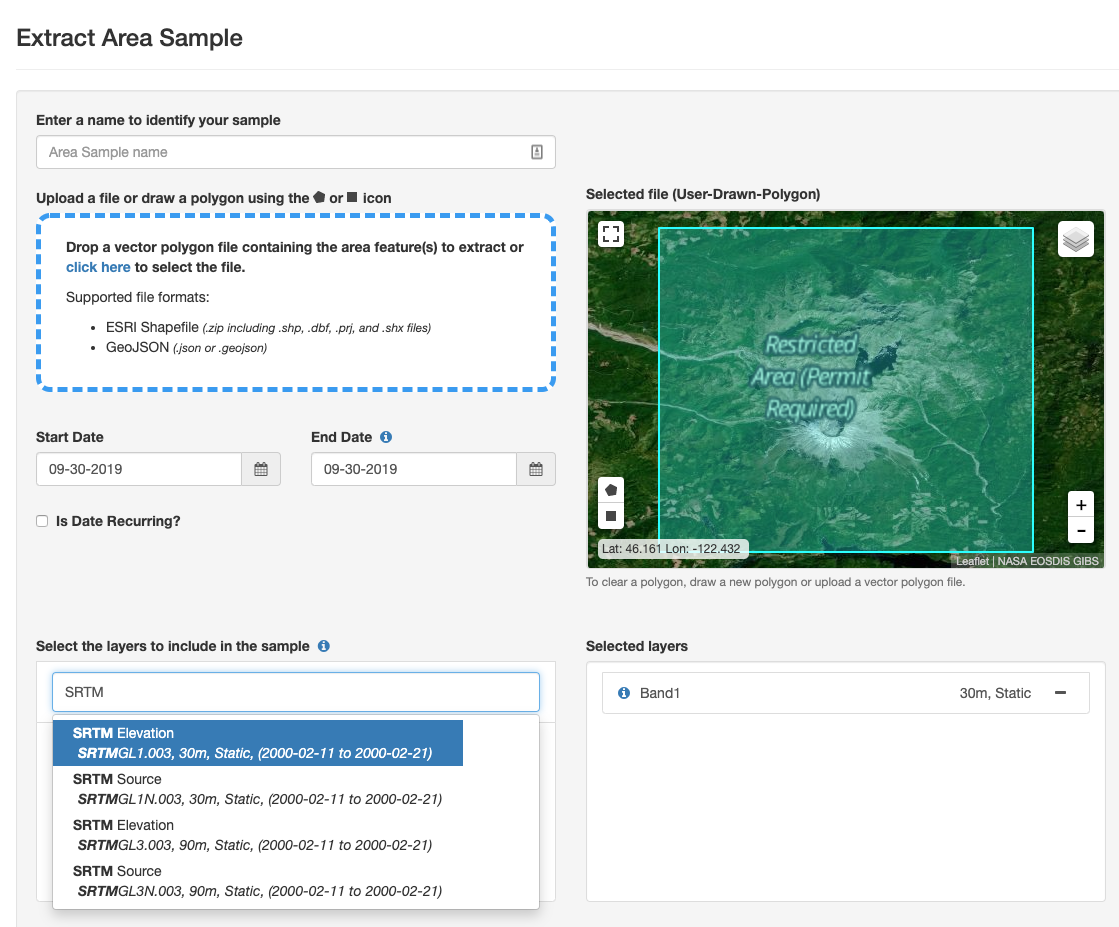
# )[0].plot(["wiggles", "shotgather"])Salvus natively also supports surface topography elevation models available via the AppEEARS webservice. The AppEEARS project is run by the USGS, and offers "a simple and efficient way to access and transform geospatial data from a variety of federal data archives". For our purposes we're interested in data stored from NASA's Shuttle Radar Topography Mission, or SRTM. This project provides elevation measurements with reference to the WGS84 ellipsoid at 30m resolution for most of the globe. Access to the data is provided through a simple graphical user interface, as shown in the figure below. To use AppEEARS yourself you simply need to create an account at the website and get going! The workflow we present below is generic, and can be applied to any UTM domain for which SRTM data is available.
Once an AppEEARS request is made, the data will be fetched and you will get an email informing you that it is ready for download. The download composes of at least two files:
- A
.jsonfile containing the parameters of your request, as well as the spatial domain for which it was made - A NetCDF file containing the SRTM data at the resolution you requested.
The
Domain constructor within Salvus project can recognize AppEEARS request files, and can use them to set automatically set up a cartesian domain in the correct UTM zone. We do this below. You'll notice that we supply an extra parameter: shrink_domain. This factor exists to make it easy to isotropically shrink the domain specified in the AppEEARS request. Specifying such a value is necessary in our case as the mesh we create will eventually require absorbing boundary layers to be attached. If these layers extend past the boundaries of the topography files, we should expect some artefacts in the interpolation of the topography. Shrinking the domain here provides an easy way to ensure that the topography model is still valid for the absorbing region.domain_appeears = sn.domain.dim3.UtmDomain.from_appeears_request(
json_file="./data/appeears.json", shrink_domain=10000.0
)
domain_appeears.plot()
Just as the domain has a constructor which can take an AppEEARS request, the actual topography data can also be initalized using a similar interface. Here we use the second file passed to us from AppEEARS, which is the NetCDF file containing the actual topography data. This inteface also takes a few additional parameters which determine how the topography is read and constructed. Here we pass
decimate_topo_factor which only reads every "nth" value in the data file. Since we will be working with relatively low-frequency simulations we will not need topography data every 30m. Decimating the data allows us to work with a smaller file in memory with almost no effect on the final mesh. We also pass the utm object stored within the Domain. The object is a pyproj.Proj projection object which defines how we transform the coordinates in the APPEEARS request to those in our UTM domain.topo_appeears = (
sn.topography.cartesian.SurfaceTopography.from_appeears_request(
name="appears_topo",
data="./data/sthelens.nc",
decimate_topo_factor=100,
utm=domain_appeears.utm,
)
)
topo_appeears.ds.dem.T.plot(aspect=1, size=7)<matplotlib.collections.QuadMesh at 0x7f44a1a189d0>

With these two objects you could reproduce the whole tutorial using AppEEARS DEM data.

PAGE CONTENTS