This documentation is not for the latest stable Salvus version.
Sometimes it is useful to interact with third-party meshing software. This
may be case, for example, when using meshes based on CAD models. Salvus
supports the use of such meshes, and has automated readers for a collection
of open-source mesh formats. In this tutorial we'll give an overview of the
currently supported formats along with an example of their use. The first
thing to do of course is to import the required Python packages.
%matplotlib inline

from pathlib import Path

import h5py
import matplotlib.pyplot as plt
import numpy as np
import os
import salvus.mesh.unstructured_mesh as um
from salvus.flow import api
from salvus.flow import simple_config as sc
from typing import List

SALVUS_FLOW_SITE_NAME = os.environ.get("SITE_NAME", "local")
Also, to make our lives a bit easier, we'll write a few short functions that
will help us quickly generate Salvus inputs as we proceed
def get_basic_source(
    *, frequency: float, physics: str, location: List
) -> sc.source:
    """Gets a simple physics- and dimension-dependent source.

    Args:
        frequency: Center frequency of the (Ricker) wavelet.
        physics: Physics of the source.
        location: Location of the source.

    Returns:
        SalvusFlow source object appropriate for the specified physics.
    """

    l = location
    src = sc.source.cartesian
    s = sc.stf.Ricker(center_frequency=frequency)
    if physics == "acoustic":
        return src.ScalarPoint3D(
            x=l[0], y=l[1], z=l[2], f=1, source_time_function=s
        )

    return src.VectorPoint3D(
        x=l[0], y=l[1], z=l[2], fx=1.0, fy=1.0, fz=0.0, source_time_function=s
    )
Exodus is one of the more common third-party mesh formats, and SalvusMesh
can read Exodus files natively. In the following example we'll read some
Exodus meshes into Salvus and run some simulations. We'll focus on two use
cases: a purely elastic simulation, and a coupled fluid-solid simulation.
# Read mesh from Exodus file.
mesh = um.UnstructuredMesh.from_exodus("./data/glass.e")

# Find the surface of mesh.
mesh.find_surface(side_set_name="surface")

# Mark simulation as elastic.
mesh.attach_field("fluid", np.zeros(mesh.nelem))

# Attach parameters.
pars = {"VP": 5800, "VS": 4000, "RHO": 2600}
template = np.ones_like(mesh.get_element_nodes()[:, :, 0])
for key, value in pars.items():
    mesh.attach_field(key, template * value)

# Visualize.
mesh
<salvus.mesh.unstructured_mesh.UnstructuredMesh at 0x7f5218dea4d0>
# Set up simulation.
w = sc.simulation.Waveform(
    mesh=mesh,
    sources=get_basic_source(
        frequency=100.0, physics="elastic", location=[0, 0, 70]
    ),
)

# Generate a movie.
w.output.volume_data.format = "hdf5"
w.output.volume_data.filename = "movie.h5"
w.output.volume_data.fields = ["displacement"]
w.output.volume_data.sampling_interval_in_time_steps = 100

# Validate simulation parameters.
w.validate()api.run(
ranks=2,
get_all=True,
input_file=w,
site_name=SALVUS_FLOW_SITE_NAME,
output_folder="output",
)SalvusJob `job_2403150914627285_8d333ca5bf` running on `local` with 2 rank(s). Site information: * Salvus version: 0.12.16 * Floating point size: 32

* Downloaded 42.1 MB of results to `output`.
* Total run time: 7.61 seconds.
* Pure simulation time: 7.25 seconds.
<salvus.flow.sites.salvus_job.SalvusJob at 0x7f520baa1d50>
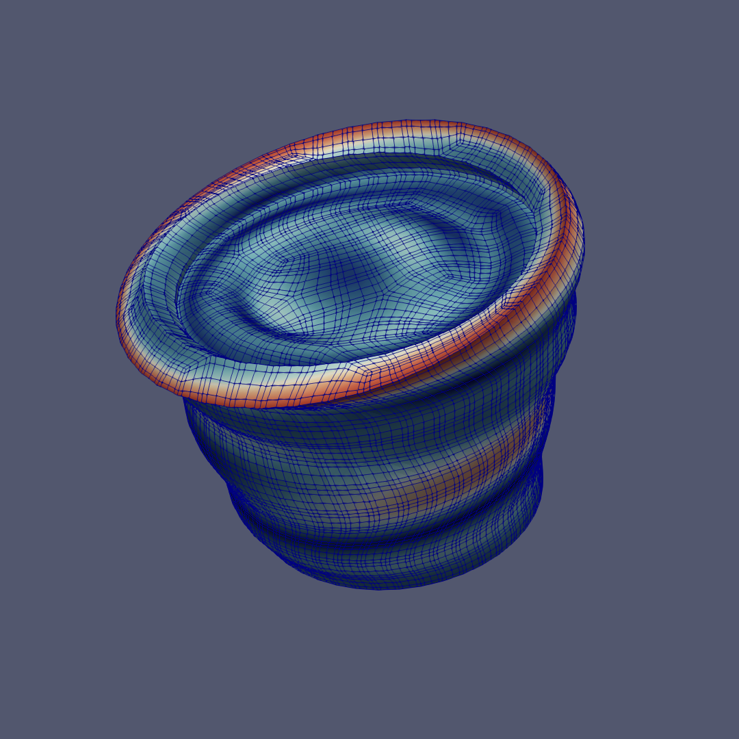
Snapshot of the magnitude of dynamic elastic displacement, visualized using Paraview and the output
.xdmf file.# Read mesh from Exodus file.
mesh_solid = um.UnstructuredMesh.from_exodus("./data/solid.e")
mesh_fluid = um.UnstructuredMesh.from_exodus("./data/fluid.e")
# Mark fluid and solid elements.
mesh_solid.attach_field("fluid", np.zeros(mesh_solid.nelem))
mesh_fluid.attach_field("fluid", np.ones(mesh_fluid.nelem))
# Attach parameters (elastic).
pars = {"VP": 5800, "VS": 4000, "RHO": 2600}
template = np.ones_like(mesh_solid.get_element_nodes()[:, :, 0])
for key, value in pars.items():
mesh_solid.attach_field(key, template * value)
# Attach parameters (acoustic).
pars = {"VP": 1500, "VS": 0, "RHO": 1000}
template = np.ones_like(mesh_fluid.get_element_nodes()[:, :, 0])
for key, value in pars.items():
mesh_fluid.attach_field(key, template * value)
# Combine both element blocks.
mesh = mesh_solid + mesh_fluid
# Find the surface of mesh.
mesh.find_surface(side_set_name="surface")
# Visualize.
mesh
<salvus.mesh.unstructured_mesh.UnstructuredMesh at 0x7f520b218f90>
# Set up simulation.
w = sc.simulation.Waveform(
    mesh=mesh,
    sources=get_basic_source(
        frequency=100.0, physics="acoustic", location=[0, -30, 70]
    ),
)

# Set your simulation length here.
# w.physics.wave_equation.end_time_in_seconds = ?

# Generate a movie.
w.output.volume_data.format = "hdf5"
w.output.volume_data.filename = "movie.h5"
w.output.volume_data.fields = ["displacement", "phi_tt"]
w.output.volume_data.sampling_interval_in_time_steps = 100

# Validate simulation parameters.
w.validate()api.run(
ranks=2,
get_all=True,
input_file=w,
site_name=SALVUS_FLOW_SITE_NAME,
output_folder="output_coupled",
)SalvusJob `job_2403150914407299_5c88f8a086` running on `local` with 2 rank(s). Site information: * Salvus version: 0.12.16 * Floating point size: 32

* Downloaded 31.1 MB of results to `output_coupled`.
* Total run time: 6.86 seconds.
* Pure simulation time: 6.61 seconds.
<salvus.flow.sites.salvus_job.SalvusJob at 0x7f520b67f490>
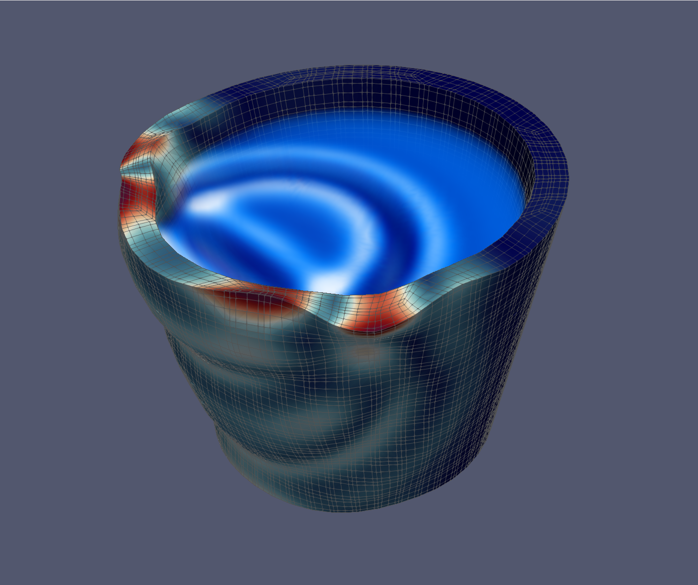
Snapshot of the magnitude of dynamic elastic displacement and the acoustic pressure, visualized using Paraview and the output
.xdmf file.
PAGE CONTENTS