Mondaic - Full Waveform Solutions

This tutorial is presented as Python code running inside a Jupyter Notebook, the recommended way to use Salvus. To run it yourself you can copy/type each individual cell or directly download the full notebook, including all required files.

Download Jupyter Notebook [21.47 MB]

In this notebook we'll go over how to add 3-D models of material parameters, topography, and bathymetry to a project. We'll then setup a simulation, and model one of the events we've selected in the previous notebook. Finally, we'll take a look at some initial comparisons to real data, and see how we can easily visualize the simulation output. Let's get started!

First, let's set up some variables that will persist while the notebook runs. These essentially determine the size of the simulations we will run, and have been chosen to respect the computational resources available in the workshop. If you have access to a more powerful machine, feel free to scale these up (shorter periods). Alternatively, if you are running on a laptop, it may be beneficial to scale them down (longer periods). For the current tutorial, we recommend keeping the settings as they are so we can keep simulations times short and to the point.

Copy

import os

PROJECT_DIR = "project_dir_central_europe"

MIN_PERIOD = 70.0
MAX_PERIOD = 120.0
SIMULATION_TIME_IN_SECONDS = 500.0

RANKS_PER_JOB = 4
SALVUS_FLOW_SITE_NAME = os.environ.get("SITE_NAME", "local")
period_band_name = f"{int(MIN_PERIOD)}_{int(MAX_PERIOD)}_seconds"

Now, let's import the Salvus namespace to get ahold of the necessary tools...

Copy

from salvus import namespace as sn

...and below we'll open up the project we created in Part 1. This project contains a snapshot of the current "state" of our work. Within it are the organized real data we looked at in Part 1, along with the definition of our domain (a SphericalChunk domain centered on Europe, in this case). The use of the project in this way is meant as an organizational tool. Instead of having large, monolithic notebooks, scripts, and configuration files, multiple smaller notebooks can be used instead. This helps keep workflows concise and focused. Additionally, since the project is just saved transparently on disk, it can be shipped to colleagues and other researchers.

Copy

p = sn.Project(path=PROJECT_DIR)

One of the most powerful features of the spectral-element method is its ability to accurately simulate seismic events through heterogeneous models, both in terms of material coefficients and domain geometry. SalvusProject currently distinguishes three types of models:

Material models
Topography models
Bathymetry models

Let's see an example of each of these in turn below.

For the purpose of this tutorial, we'll use the 3-D mantle model s362ani (Kustowski et al., 2008), which can be downloaded directly from the IRIS Earth Model Catalogue (EMC). We've gone ahead and pre-downloaded this model for you, and placed it in the data subdirectory. Before using the model later on for a simulation, we'll first have to add it to our project as below.

Copy

p.add_to_project(
    sn.model.volume.seismology.GenericModel(
        name="s362_ani", data="data/s362ani.nc", parameters=["VSV", "VSH"]
    )
)

You may have noticed here that we added the model using the GenericModel function -- in contrast to the possible MantleModel or CrustalModel options. This is, again, due to the relatively limited resources present on the training cluster. While GenericModel will interpolate the provided model without any consideration of radial discontinuities, the other two classes will ensure that interpolation only happens in the specified regions. In the standard use case we can use multiple 3-D models in a simulation, within and across target regions.

The inclusion of realistic surface topography is a common requirement for regional-to-global scale simulations. On the Mondaic website, topography files integrating data from EGM2008, Earth2014, and Crust1.0 can be downloaded, with a maximum spatial resolution of 1.8 km globally. These data are pre-processed to avoid aliasing, and the proper resolution model will be used depending on the resolution of the mesh. For use cases that require even higher-resolution topography, we recommend using Salvus' UtmDomain, but that is beyond the scope of this tutorial. We can register this topography model with the project as below.

Copy

p.add_to_project(
    sn.topography.spherical.SurfaceTopography(
        name="surface_topography", data="data/topography.nc"
    )
)

Seismic waves are affected by the presence of oceans, and at higher frequencies it becomes necessary to simulate a coupled fluid-solid system. While this is possible in Salvus, at the frequencies we're interested in approximating the effect of the oceans by a mass loading term is sufficient and practical for this tutorial. Bathymetry models are derived from the same data source as the topography models above, and can be added to a project in a similar manner.

Copy

p.add_to_project(
    sn.bathymetry.spherical.OceanLoad(
        name="ocean_bathymetry", data="data/bathymetry.nc"
    )
)

We now have almost all the essential ingredients required to set up our first forward simulation, which we'll do in the cell below by defining a SimulationConfiguration. It's a bit verbose, so let's go through the settings one by one! First, let's start with some fundamental ones.

name: This one is self-explanatory. SalvusProject will use this name to refer to this specific set of simulation parameters from now on.
max depth in meters: This one is also pretty simple. We want to truncate our domain at a certain depth.
elements per wavelength: This one is a little more subtle, and controls the accuracy of our simulation. We usually say that one element per minimum wavelength in the mesh is sufficient for regional -> global scale applications, but in some circumstances more accuracy might be desired. Here we set it to 1.25, resulting in some minor over-resolution. Note that, like frequency, 3-D simulations scale with this value to the power of 4!
min period in seconds: This parameter is intimately tied to the previous one, and specifies at which frequency the elements per wavelength refers.

After these first four, we get to the parameters related to the models we've defined above.

model configuration: A "configuration" in this parlance is a collection of individual components which are used together. A "model configuration" is then the final, concrete model which we will interpolate onto our mesh. The only required argument here is "background model", which we set to PREM, but in our case we'll attached the 3D s362_ani model as well. If we had had crustal or mantle models in addition, we could just add them to the array here.
topography configuration: Similar the model configuration, this is where we specify what topography model to use. If we had also defined Moho topography, it would enter here as well.
bathymetry configuration: Now we're getting a bit repetative. Here we specify that we do want to model bathymetry in the upcoming simulation, and that this bathymetry should be the ocean load we add to the project previously.

Next up, we specify our sources, receivers, and any additional physics that we want to simulate.

event_configuration: The event configuration has the primary purpose of adding time-dependent information to our simulation. Here we specify what source wavelet we want to use (a Ricker wavelet in this case), and also any additional parameters related to the simulation specifics. Here we'll turn on attenuation, and say that we want to simulate for 500 seconds after the centroid time.

Finally, we'll specify what kind of boundary conditions we want to use.

absorbing_boundaries: Salvus employs a damping-layer type of absorbing boundary condition, and this requires an additional buffer of elements along the relevant boundaries. We find that the performance of these types of boundaries are acceptable when 3.5 or more wavelengths propagate within the boundary region. To keep things small and manageable here though, we'll set the "number of wavelengths" parameter to 0. In this case, we fall back to a 1st order (Clayton-Enquist) boundary condition on the relevant edges.

Copy

p.add_to_project(
    sn.SimulationConfiguration(
        name="my_first_simulation",
        max_depth_in_meters=1750e3,
        elements_per_wavelength=1.25,
        min_period_in_seconds=MIN_PERIOD,
        model_configuration=sn.ModelConfiguration(
            background_model="prem_ani_one_crust", volume_models=["s362_ani"]
        ),
        topography_configuration=sn.TopographyConfiguration(
            "surface_topography"
        ),
        bathymetry_configuration=sn.BathymetryConfiguration(
            "ocean_bathymetry"
        ),
        event_configuration=sn.EventConfiguration(
            wavelet=sn.simple_config.stf.GaussianRate(
                half_duration_in_seconds=2 * MIN_PERIOD
            ),
            waveform_simulation_configuration=sn.WaveformSimulationConfiguration(
                end_time_in_seconds=SIMULATION_TIME_IN_SECONDS,
                attenuation=True,
            ),
        ),
        absorbing_boundaries=sn.AbsorbingBoundaryParameters(
            reference_velocity=3700.0,
            number_of_wavelengths=0.0,
            reference_frequency=1.0 / MIN_PERIOD,
        ),
    )
)

That was quite a lot of information, but with our simulation defined we're almost ready to go. Before we fire stuff of though, let's visualize what we've setup. Spend some time exploring and looking at the different options.

Copy

p.viz.nb.simulation_setup("my_first_simulation", events=p.events.list())

[2024-03-15 09:36:32,994] INFO: Creating mesh. Hang on.
Interpolating model: s362_ani.

<salvus.flow.simple_config.simulation.waveform.Waveform object at 0x7fade58a70d0>

Remember, all the events and receivers shown above were defined in the previous notebook, and correspond to real GCMT events and seismometers. You may have noticed a bunch of progress bars popping up with the text "locating n items"... what is going on here? Well, in a general, deformed domain, the actual locating of source and receiver positions is a non trivial task. For instance, the absolute location of the mesh surface is dependent on the topography model, which is dependent on the resolution of the mesh ... you get the picture. To deal with this, Salvus solves an auxiliary optimization problem to ensure that the location of each source and receiver is exact with respect to the mesh surface. This means that if a source is 20km below the surface, it will be placed as such -- regardless of the complexity of the topography.

Now we're ready for launch. Below we'll leverage SalvusFlow to manage job submission and monitoring for us. As this is a tutorial, we'll likely be running jobs locally, but the same workflow applies regardless of where the computations will take place -- all that is required is to change the site_name parameter. If the site is remote, i.e. a supercomputing cluster, SalvusFlow will handle all the uploading and downloading of input files for you, as well as monitor the queue for job completion. You'll be informed when everything is done, and when the data is available for analysis.

Note below the dictionary we pass to extra_output_configuration. This allows us to easily request specialized outputs for one-off simulations, and in this case we'll use it to output snapshots of the wavefield propagating along the mesh's surface. We'll use this in the final cells to open and visualize in Paraview.

Well: let's pick an event in the center of the domain, and get to work!

Copy

p.simulations.launch(
    events="event_CRETE_GREECE_Mag_6.15_2015-04-16-18-07",
    simulation_configuration="my_first_simulation",
    site_name=SALVUS_FLOW_SITE_NAME,
    ranks_per_job=RANKS_PER_JOB,
    extra_output_configuration={
        "surface_data": {
            "side_sets": ["r1"],
            "sampling_interval_in_time_steps": 100,
            "fields": ["velocity"],
        }
    },
)

[2024-03-15 09:36:34,415] INFO: Submitting job ...
Uploading 1 files...

🚀  Submitted job_2403150936510124_81e594dcaf@local

We can check the status of running simulations by calling the query command as below. Who will win? The block=True parameter informs Salvus that we don't want to continue until our simulations are finished, as opposed to a more asynchronous mode of operation.

Copy

p.simulations.query(block=True, ping_interval_in_seconds=5)

True

While the job is running, its worth exploring what happened during the last few cells. When we made the call to launch and/or query, we're invoking a call through SalvusProject to SalvusFlow. Before any computations happen, SalvusProject checks whether or not the relevant input files exist for a given simulations configuration, and creates them if they do not. The input files are then shipped over to the compute server (which may be local), and the job is run with SalvusCompute. Finally, everything is copied back to the host machine. All of this is done lazily, and if SalvusProject detects that this exact same configuration has been run before, it will simply return the already-computed data to you, rather than launching off another simulation. We'll see the benefits of this in the next few notebooks.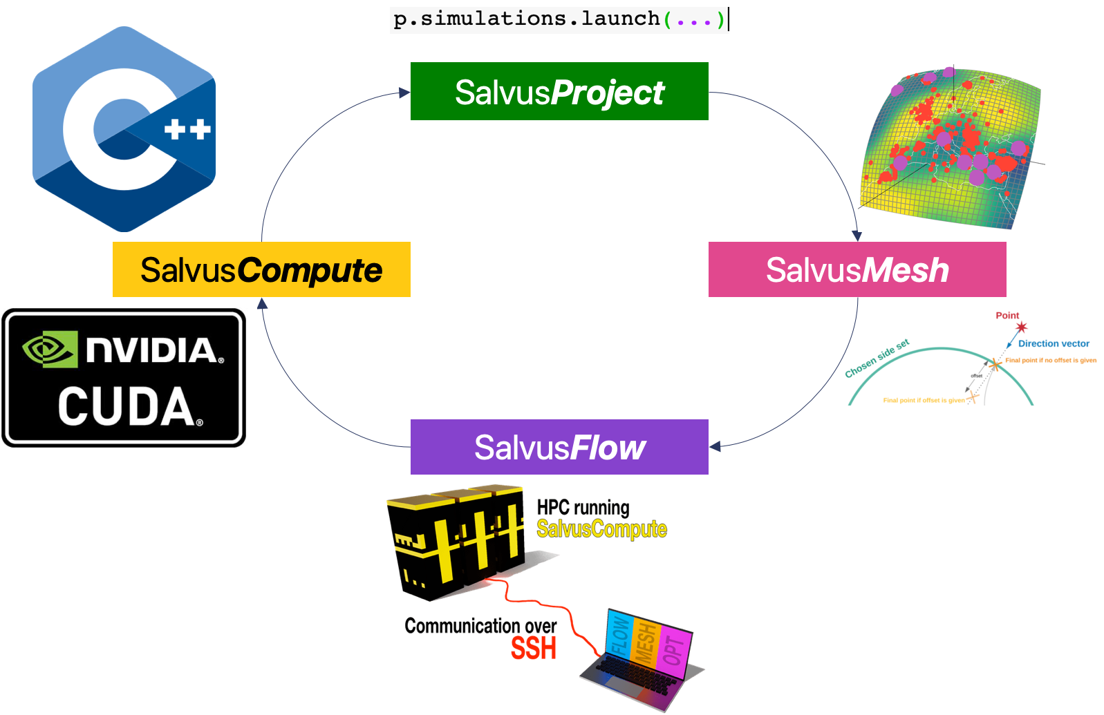

While an automated workflow is great for many batched applications, it is sometimes desirable to break out of it and inspect output files manually. This is especially relevant here with the surface output we've saved. In general, these files can get very large, and it would be very inefficient to always transfer them. If we want to access the raw data from a simulation, we can simply copy it from the simulation output directory. The receivers are stored in the standard ASDF format, which works natively with Obspy. In this case, we'll also download the surface output that we specified above. Try out copying the output directory to your local machine, and opening the resulting XDMF file following these instructions.

Copy

print(
    "Rsync (or scp) me!",
    p.simulations.get_simulation_output_directory(
        "my_first_simulation",
        event="event_CRETE_GREECE_Mag_6.15_2015-04-16-18-07",
    ).absolute(),
)

Rsync (or scp) me! /tmp/tmpzmy1cfxt/project_dir_central_europe/EVENTS/event_CRETE_GREECE_Mag_6.15_2015-04-16-18-07/WAVEFORM_DATA/INTERNAL/34/6a/803cc38f496a

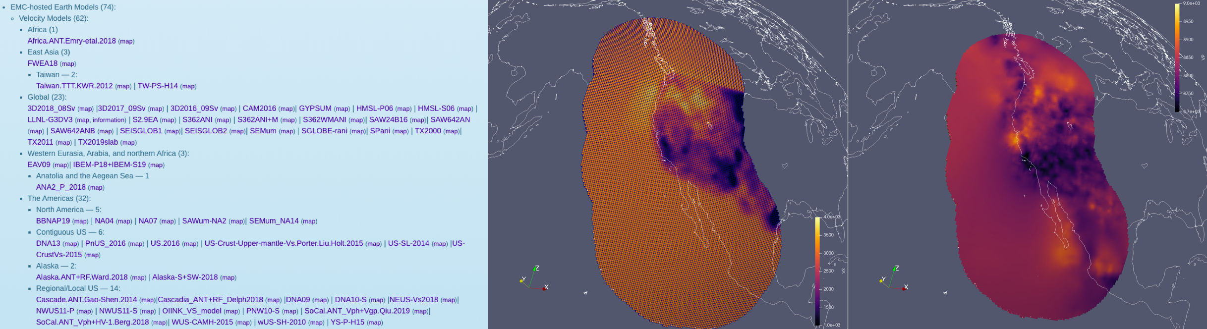
The .nc files we used in this tutorial are in fact the same convention that is used by the IRIS Earth Model Catalogue (EMC). This means that many of the models stored in the EMC can be downloaded and used directly in Salvus! Unfortunately, there is no standard parameter set stored in the EMC, and we've found that not all the files actually conform to the required convention. Nevertheless, with some minimal processing, you can have the public library of 3-D Earth models at your disposal to run simulations through. The picture below show a successful attempt at including 3 distinct 3-D Earth models (crust, mantle, cascadia) for a region along the US west coast.